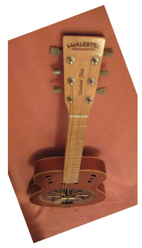
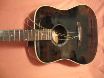
Data from a blueprint for a Beard Resonator Guitar.
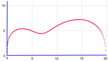
This equation, the sum of several sine functions multiplied by a fourth-order polynomial and two arctangent functions, is designed to trace the outline of an acoustic guitar. The parameters A through S are unique to each instrument and are discovered by fitting the equation to an instrument with "curve-fit" software. A large number of parameters is necessary in order that this mathematical curve precisely fit the guitar outline. A value for the body length of the guitar, BL, also unique to each insrument, is entered directly into the equation since it is not altered during a curve fit.
The equation is fairly universal, meaning that it will fit the outline of just about any guitar, provided, of course, that proper values for the parameters can be found. For some instruments a few more sine functions have been included, which increases the number of parameters and makes for a better fit. The polynomial is necessary, but increasing its order does not produce a better fit, nor does decreasing the order improve the fit.
The arctangent functions also are required. As a matter of fact, they are the key to making the equation work. Their purpose is to pin the curve at the endpoints of the instruments. Without the arctangents the curve tends to splay-out at the ends.
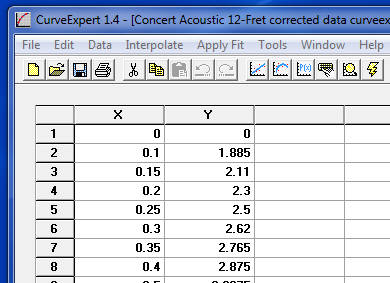
At first I used the excellent and highly recommended (by me) program Curve Expert Basic to find the parameters, and later Curve Expert Pro. One advantage these programs have over other curve-fit programs is that they will allow a large number of parameters. Curve Expert Basic will fit a curve with up to 19 parameters; Pro will allow an infinite number. I have found that these programs will produce a fast and sure fit. I could not have developed the equation without Curve Expert.
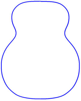
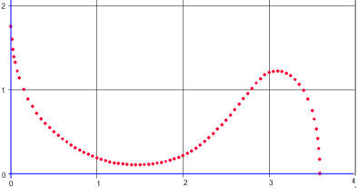
To obtain data for an instrument, the guitar outline is traced onto a sheet of graph paper with the half-pencil technique for a precise curve. The center line of the guitar lies along the x-axis with the origin of the coordinate system at the neck; the y-values, then, describe the body half-width.
To find the parameters an initial set is selected, the equation is then evaluated and compared with the set of data points which describe the outline. If necessary, the parameters are altered, the equation is re-evaluated and again compared with the data. Many iterations (perhaps hundreds) may be required to produce a close fit between the curve and the data. The initial parameters were complete guesses; after many stabs in the dark a solution was eventually stumbled upon.
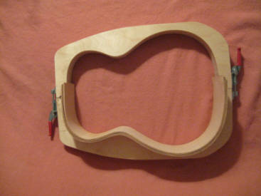
The original point series data for the guitars described here come either from an instrument itself, a blueprint, or a body mold. The outline of the guitar is traced onto a sheet of graph paper using the half-pencil technique to obtain a precise curve. The center line of the guitar lies along the x-axis with the origin of the coordinate system at the neck; the y-values, then, describe the body half-width.
Data for the Gibson J40 Dreadnought, for example, was taken for the most part at 0.05" increments along the x-axis; closer together near the ends where the curve is quite steep. Two hundred thirty three pairs of (x,y) data points were recorded for this instrument; such a large number of points is needed for a smooth curve fit.
About the same number was obtained for all of the curves described here.
The curves for several instruments, including the bass side of a Les Paul, are on the following pages with the parameters given in tables. To plot the curves for these instruments, just enter the equation into a suitable graphing program and copy and paste the parameters (and the body length) into the program. Since the curve is quite sensitive to slight changes in the parameters, the parameters are written to seven significant figures. Rounding to five or fewer figures will distort the curve. When printing the graph be sure that the scales along the x- and y- axes are identical.
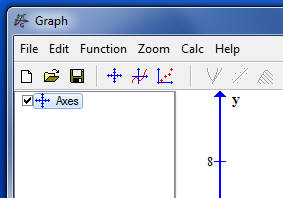
A suitable graphing program is Graph; it has the advantages of both being a free download, and also can be imbedded into a "Word" document. Logger Pro is a specialty graphing program used in many school science labs, the utility of which is enhanced because of its many available functions - including those of calculus. It may be possible to select equation (1) from this page as text, copy it, and paste it directly into a graphing program. Graphing programs generally do not require the "y =" part of the equation.
y = (A*sin(B*x + C) + D*sin(E*x + F) + G*sin(H*x + I) + J*sin(K*x + L)) * (M*x^4 + N*x^3 + O*x^2 + P*x + Q) * (3.0 - arctan(R*x)) * arctan(S*(BL - x)) (2)
To use the equation to produce a curve for another guitar, it might help to identify which of the outlines on these pages the guitar most closely resembles. The parameters given here could be used as effective initial guesses for an efficient curve fit. If the attempted fit does not converge towards a solution, try another set of parameters.
The bass side of the Les Paul resembles the shape of an acoustic guitar so the fit of that side is straightforward, although mirrored in the coordinate system used here. However, the treble side cutaway presents a problem. The curve fit programs will not allow a curve to turn over on itself; that is, you can't have two y-values for any given x-value. To solve this problem the cutaway is turned upright and fit separately from the rest of the side. The equation is modified so that one of the arctangent functions pins the curve at the now upright neck. The first arctan term in equation (1) is replaced by (3.0 - arctan(R*x)). This cutaway curve can then be conjoined to the bass side curve to produce the treble side of the Les Paul.
y = (A*sin(B*x + C) + D*sin(E*x + F) + G*sin(H*x + I) + J*sin(K*x + L)) * (M*x^4 + N*x^3 + O*x^2 + P*x + Q) * arctan(R*x) * arctan(S*(BL - x)) (1)
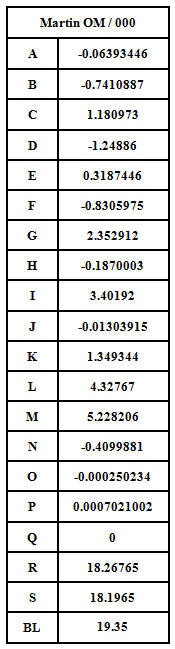
Parameters for a Martin OM / 000 Guitar
Graphing programs usually offer a number of additional features, such as the line length calculator in Graph. On the other hand, Logger Pro does not have a built in line length calculator, but it does have both the derivative and integral functions available. With these the path length can be calculated. If m(x) is the derivative of y(x), namely,
then the line length, L, from the origin to the end of the guitar can be found by the integral
where dx is the differential of length along the x-axis. In Logger Pro language,
integral(sqrt(1+derivative(y)^2))
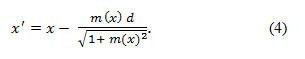
The curves described above are fit to the outside surface of the guitar body, of course. A curve which fits the inside surface of the guitar's side may be required; for example, an accurate calculation of an acoustic guitar's internal volume will require knowledge of the area of the top or back plate up to this inside curve. Finding the inside curve requires calculating a couple of derivatives. These derivative functions might be obtained explicitly using calculus, but this is not really necessary with these modern graphing programs like Logger Pro since a numerical solution is sufficient. First, define d as the side thickness and calculate x' using the equation
For the instruments here, a nominal side thickness of 0.085" has been used.
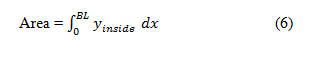
Now the area under the inside curve is
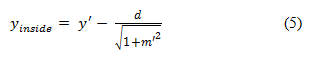
Now, calculate a new set of points, y’, using equation (1), but substitute x’ in for x. If m(x)’ is the derivative of y’, then the inside curve is
y = (A*sin(B*x+C) + D*sin(E*x+F) + G*sin(H*x+I) + J*sin(K*x+L)) * (M + N*x + O*x^2 +P*x^3 + Q*x^4) * atan(R*x) * atan(S*(BL-x))