We see from equation (32) that 𝜂 is on the order of 1.  Eccentricities of planetary orbits are less than .25 (typically much less) so the coefficients which multiply the sine functions, εk/k! are on the order of, or less than, 10^-5 for terms in ε⁵ and higher, so they are probably small enough that we might neglect those terms.  Let us do so, and write ξ₀ for ξ in the first term on the right-hand-side, and then substitute in for 𝜂 and solve for ξ.

HOME

Page 1  Elliptical Orbits

Page 2  Time Dependency

Page 3  Kepler’s Equation

Physics Home

Kepler’s Equation, Part 2

Kepler’s Equation, Part 2

D)  Approximate Solution

How to Use Kepler’s Equation, continued.

Then plugging this into Kepler’s equation,

and simplifying gives us

Expand sin(ξ) in a power series

and substitute the right-hand-side of equation (32) into the right-hand-side (only) of the series

We will need ξ₀ and 𝜂 so we may as well solve for these now,

Move the first term of the series to the left-hand-side; then using the sum-of-two-angles identity for the sine function we have

On the right-hand-side of this we have those two square brackets which have ε and       mixed-up together, so we may deal with them by change-of-variable.  Define ξ₀ and 𝜂 with these expressions:

Therefore,

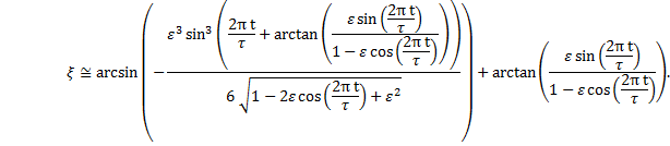
With these, the left-hand-side of our approximation becomes

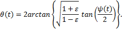
To solve Kepler’s equation with this approximation, first calculate ξ with this last expression and use equation (31) to find ψ.  The rest is duck soup; for example, to calculate θ use

Now substitute in for ξ₀ and

Thus an approximate solution might be found if

-----------------------------------------------------------------------------------------------

Approximate Solution In Logger-Pro:

Mercury

 

First, follow this path, beginning with the tab at the top of Logger-Pro,

Data>>User Parameters>>Add. 

Enter the values and name any constants which might be used; for example, ε (“epsilon”, .0256), τ (“tau”, 87.969) and a (“a”, 5.7871E10).  Note that “pi” is already entered.

Next, Logger-Pro requires a set of numbers to plot along the x-axis; these numbers may be generated following this path:

Data>>New Manual Column>> Generate Values.

For just over one Mercury orbit, let 0 < t < 100 days, in, say, 0.1 increments.  Copy-and-Paste these newly generated numbers into the X-column; rename the column “t”, with units “day”.  By default the X-column is placed along the graph’s abscissa, but another column may be substituted by double-clicking the cursor on the graph, clicking on the tab “Axes Options” and selecting a new “X-Axis Column”.

Now, for simplicity in calculation, each variable should be generated in its own column; follow the path:

Data>>New Calculated Column>>Column Definition.

Name the column and enter the equation in the box called “Expression”.  Note that in entering expressions, the variables are enclosed in quotation marks – this refers to the column name since calculations in Logger-Pro are made by column.  In order to place one of these columns along the ordinate of the graph, double-click on the graph, click on the tab “Axes Options” and select “Y-Axis Column”.

Using the expressions for x and y given at the top of this page, we have

so,

and

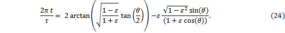
Now, the time derivative of equation (30):

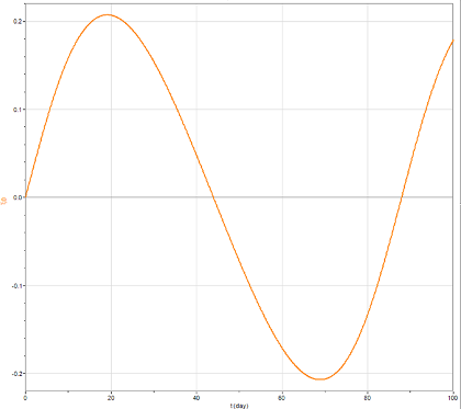
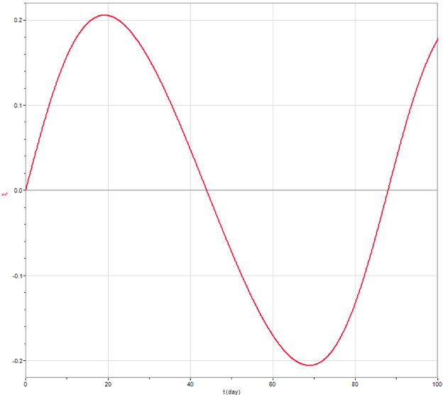
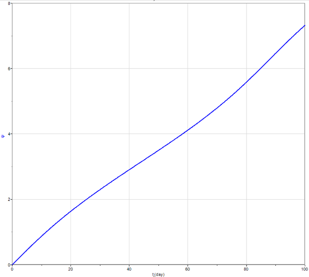
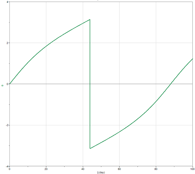
For      , enter into the “Expression” box:

2*pi*"t" /tau

For ξ₀, enter

atan(epsilon*sin("M")/(1 - epsilon*cos("M")))

For 𝜂, enter

             sqrt(1 - 2*epsilon*cos("M") + (epsilon)^2)

For ξ, enter

asin(-(epsilon^3 *(sin("M" + "ξ0"))^3)/(6*"η"))+"ξ0"

For ψ, enter

"M"+"ξ"

For θ, enter

             2*atan(sqrt((1+epsilon)/(1-epsilon))*tan("ψ"/2))

For r, enter either

             a*(1-epsilon*cos("ψ"))

or,

             a*(1-epsilon^2)/(1-epsilon*cos("θ"))

ξ₀ versus t

ξ versus t

Note that ξ and ξ₀ are about equal so our substitution was valid.

ψ versus t

θ versus t

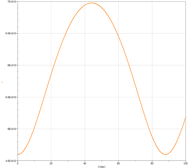
r versus t

----------------------------------------------------------------------------------------------------------------------------------

Two Last Things – Velocity and Acceleration

 

 

What is the speed of a planet?  Naturally, we write

Rearrange,

and substitute into the expression for v²

Now substitute in r/a = (1-ε cos(ψ)),

or

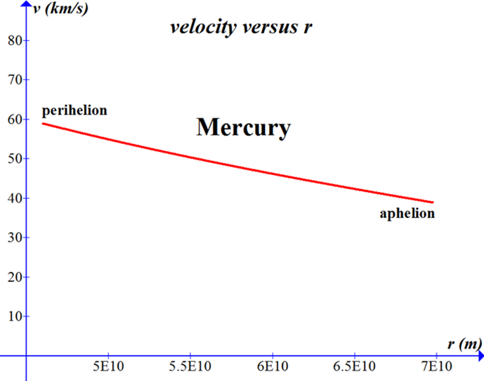
which we could simplify with Kepler’s Third law, if we wish – but we don’t, so let’s graph it.

The values of velocity at the endpoints of this curve match the aphelion and perihelion velocities taken from the NASA page and given in the table on page 1.

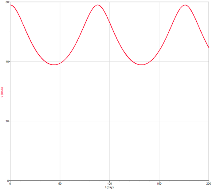
Velocity as a function of time for Mercury, that is, equation (34) with r(t) plugged in to give v(t).

Velocity in Polar Coordinates

 

 

Equation (8) is an expression for the velocity vector,

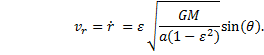
So, we can immediately write the radial component of the velocity, namely,

Recalling equation (25’),

we take the derivative

and use the expression for dθ/dt from equation (10),

which we may substitute,

Substituting in for r² we can simplify,

If you haven’t written an expression for L in terms of a and ε, now is the time to do so:

This gives us the magnitude of the radial velocity in terms of θ.  When we graph this we shall insert θ(t) for the time dependence.

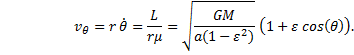
We also have the tangential component of velocity, namely,

and the magnitude of the velocity is

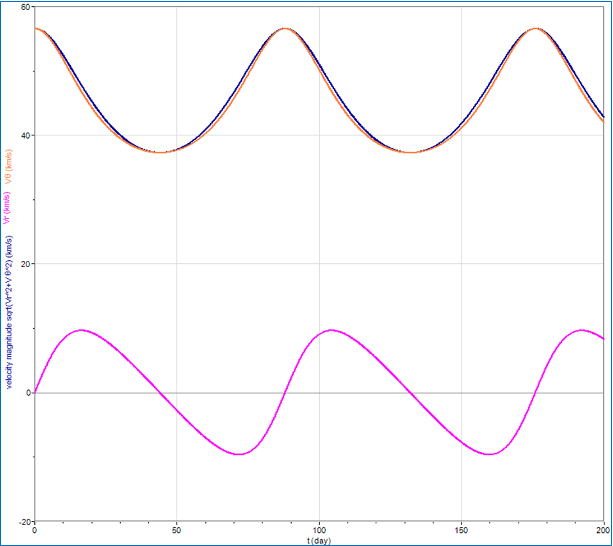
Mercury

Graphs of v_r, v_θ and v versus time

Violet,    Radial component of velocity                 Orange,    Tangential component of velocity                     Blue,    Velocity Magnitude

The magnitude is, of course,

Velocity in Cartesian Coordinates

 

 

Still on the subject of velocity, we can write the x-and y-components.  Equation (9) on Page 1 gives us the expressions to begin with,

Acceleration

 

 

Enough with the velocities.  Let us turn our attention to acceleration.  The time derivative of equation (8) gives us the acceleration,

The gravitational force is in the radial direction only so we know that there is no tangential acceleration.  One can easily show this last term is identically zero.  Reiterating, the expression for dθ/dt is

so now we can see cleary that the second derivative in the last term on the right-hand-side of a is

The time-rate-of-change of the unit vectors has been determined previously,

and,

So we can write the acceleration,

Again for Mercury, using θ(t) with these velocity expressions, I thought it would be interesting to see what the curves look like.

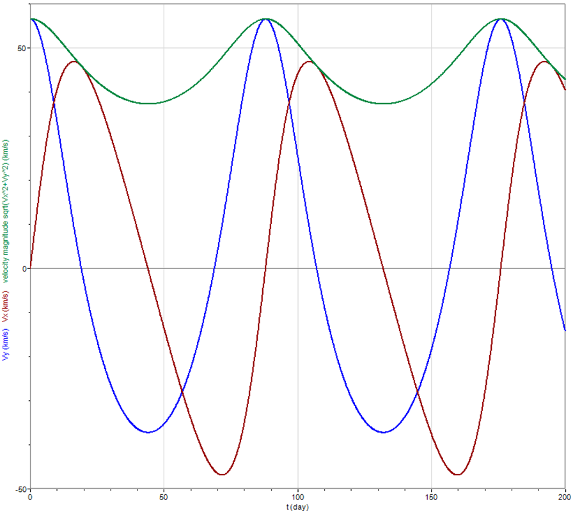
Mercury

Graphs of v_x, v_y and v versus time

Red       X-component of velocity                          Blue      Y-component of velocity                          Green    Velocity Magnitude

and thus tangential acceleration is zero.

Radial Acceleration

Let us evaluate the radial acceleration.  We have just moments ago taken the time derivative of r, equation (35).  Using the famous chain rule we may take the second derivative of r.  Recalling yet again equation (25’),

We have what we need now to write the radial acceleration:

the second derivative must then be

To remove the dependence on θ, we will leave the r² term alone and substitute in for the lone r in the parenthesis, to find

Well, there we have it: the end (except for one more graph, below) of our analysis of Newtonian mechanics as applied to elliptical planetary orbits. 

 

Of course, we know from Newton’s universal law of gravitational attraction that the magnitude of the acceleration is given by F/μ = GM / r².  If we were to substitute the relationship between L, a, and ε, viz.,

Mercury

mnealon@eosc.edu

webpages and Eos image copyright 2015 M  Nealon

Top   Kepler’s Equation Part 2

Page 1   Elliptical Orbits

Page 2   Time in Orbit

Page 3   Kepler’s Equation

with magnitude

into a_r we would see that the acceleration becomes

We won’t do this, however, since it would be a circular argument because we ultimately used Newton’s law to find that relationship between L, a, and ε (through the ever-useful work-energy theorem, naturally).

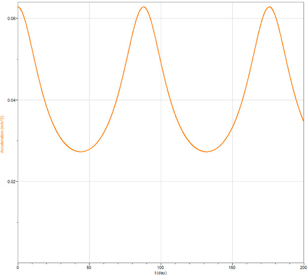
a_r versus t

We now have an approximation for the correction term.  The time dependency is via      .  After we find the solution we can check these assumptions to see whether they are warranted.  With these assumptions, then, we have