HOME

Page 1  Elliptical Orbits

Page 2  Time Dependency

Page 3  Kepler’s Equation

Physics Home

On the Question of the Planet’s Time in Orbit

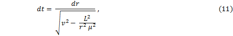
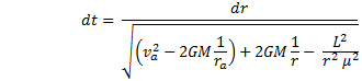
If our aim were to find the position of a planet as an explicit function of time then we would be disappointed, as the problem is transcendental, and, for that matter, intractable - meaning that we cannot invert the equation algebraically to give us r(t), and that it is not so easy to deal with.  We can, however, find time as a function of position, t(r).  To do so, let’s begin with equation (11), the relation between time and position in differential form,

and revisit the work energy theorem

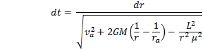
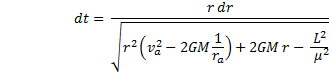
This time, let’s use the aphelion for initial conditions.  Substitute in v² and simplify.

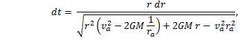
where we have substituted in the expression for the magnitude of L.  This gives us

We are using the letters a, b and c again but this time we have a new equation to solve.  Here we have

First Step Toward Solution

 

 From previous experience, we know that the chain rule for derivatives likely plays a role in solving the problem, so let’s look at the derivative of the integrand’s denominator.  The argument will be easier to follow if we use a change of variables.   Let

With this, then, and using prime notation we have

Notice that after dividing through by a, the first term on the right is the integrand, so we have

and our intermediate solution is

This gives us yet another integral to solve:

It figures.

Another Integral to Solve

 

Luckily, since this last integral is similar to the integral previously solved (in finding the elliptical orbital path) but without the lone r factor in the denominator (outside the radical), we might find the solution here by using the same technique.  That technique used derivatives – and the chain rule – to find the integrand, and, hey presto!, the integral was solved. 

 

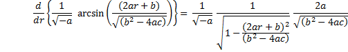
That previous integral – the one for the r dependence on θ – gave us (reverting to the variable r to avoid confusion) the solution

where, if you remember, we put in that slightly more complex argument in the arcsine; we then took the derivative of both sides.  This time as a first and simplest guess, we might try U as the arcsine argument.  If we do that, then we have

We can tell that this does not give us the solution because, as we take the derivative of the arcsine we have a square term under the radical; in this case, U to the fourth power gives us a higher order polynomial in r than we can possibly use.  This first attempt gives us a clue, however: since the solution requires a second order polynomial under the radical, if we wind up with a first order polynomial, squared, under the radical then we may have arrived at the solution.  Furthermore, we notice this:  Since the derivative of U is directly proportional to 2(2ar + b) and inversely proportional to U, the product 2UU’ is just what we are looking for: a first order polynomial!   Thus, we will try 2UU’ as the arcsine argument.  Carry the two along for the ride.

At this point let’s look at the derivative of U again and also take the second derivative.

so,

The second derivative is

Conveniently, we may substitute in for (2ar+b) to obtain

Now we are ready to put these together.

and

Therefore,

That is the solution in principle, but after all of that work solving the integral we discover that the polynomial’s coefficients are not what we need.  It’s now a simple matter of finding which combinations of constants we should include in the arcsine.  Keep in mind that whatever combinations we try, they will be squared – so we might think of putting the constants under a square root sign.  We can cancel any constant in the numerator by putting a similar factor in front of the arcsine if we need it; additionally, the chain rule we will produce another constant which might cancel another factor in the numerator.  All of this will be clear in the doing.

First of all, we see that we need to get rid of the (1-b²) term, and include a c term.  Also, we might notice that if we divide the (2ar + b) term in the arcsine by a constant, when we factor that constant out of the radical in the derivative, it multiplies the 1, and is therefore on the same line with the (2ar + b)²  and can be added or subtracted according to its sign.  The following example will illustrate the point.

 

Suppose we have something like this in the arcsine:

Integrating both sides,

In the derivative it becomes (not yet using the chain rule since we’re looking only at the radical so far)

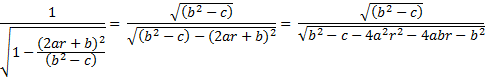
Now you can see how the b² term disappears and the c term has been introduced under the radical.  We are not there yet, so let’s try something else in the arcsine:

Again without the chain rule, that leads to

There is our second order polynomial under the radical, so we found the solution inside the arcsine, and we can see what constant we need out front.  For the complete solution, this time including the chain rule, we have 

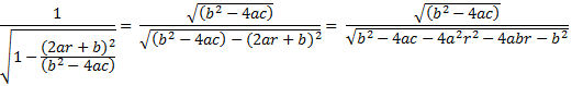
An important condition for this solution to apply to the planetary orbit is that the value of the arcsine argument must be less than 1 or greater than -1.  This means that

This solution is true

 

for     a <  0,

and    b²  > 4ac.

 

Gathering our wits together, we reiterate:

since

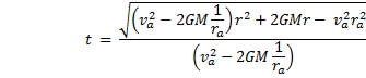
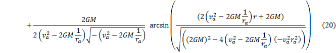
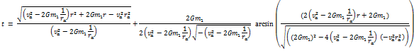
Our Final Result

 

The time dependency of the planet’s position in its orbit can be written, finally!

Integrate both sides.  We will use an indefinite integral and for the moment ignore the constant of integration.  There is no reason we cannot put in a phase shift later if we want the planet at a particular location when t = 0.

where again,

The required condition in order to use this equation is that

A second solution which works is

This solution puts the sun at the other focal point.

Solution with Initial Conditions

 

Our final result is

Regarding the coefficients, we see from the work-energy theorem that two versions of a are identically equal.  We see also that the coefficient b is independent of any orbital parameters, and, as we saw when considering the conservation of angular momentum, that the two versions of c are identically equal. 

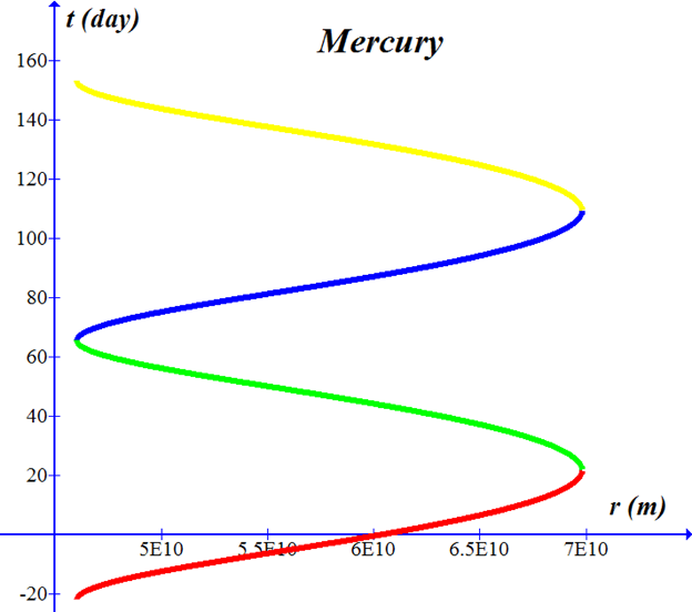
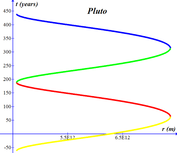
The expression for t cannot be inverted to give r as a function of t.  However, we can plot t versus r over one-half cycle of the orbit from perihelion to aphelion.  With a judicious choice of offset phases and negative signs, we can build the orbit.  We also may predict that the curve will be asymmetric, since the planet speeds up as it approaches the sun and slows down as it recedes.

======================================================================================================

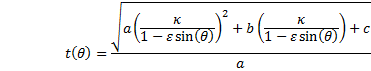
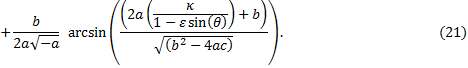
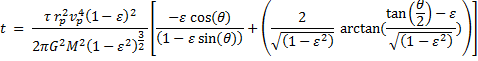
In order to obtain the time in orbit as a function of angle instead of distance, one need only substitute the expression for distance which was derived on the previous page, equation (16), into the present solution.  The expression for distance as a function of angle is

We can now rewrite equation (16) as

and for clarity, let us use a new parameter κ (see page 1 for a geometric interpretation of κ),

This may seem formidable — but it is eminently do-able, especially with modern computer graphing programs.  This is graphed below for Mercury.  Be careful when the arcsine argument is ± π/2.

Equation (19) then becomes

======================================================================================================

Graphs of t vs. r

 

First, the data.

Now the calculations.   Note that these graphs and calculations are made with m₁ rather than M.

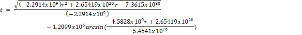
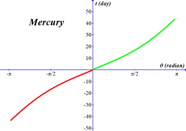
Two cycles of Mercury in its orbit.  Time in earth days on y-axis, distance from the sun in meters along the x-axis; perihelion to the left, aphelion to the right.  Note the asymetry; Mercury speeds up as it nears the sun.  Period taken from the graph is 87.5 days.

------------------------------------------------------------------------------------------------------------------------------------------

Equation written for Graph program (red curve).

 

(-sqrt(-2.2914E9*x^2+2.65419E20*x-7.3615E30)/ 2.2914E9-1.2099E6*asin((-4.5828E9*x+2.65419E20)/ 5.4541E19))/60/60/24

 

http://www.padowan.dk/

///////////////////////////////////////////////////////////////////////////////\\\\\\\\\\\\\\\\\\\\\\\\\\\\\\\\\\\\\\\\\\\\\\\\\\\\\\\\\\\\\\\\\\\\\\\\\\\\\

Mercury

 

http://nssdc.gsfc.nasa.gov/planetary/factsheet/mercuryfact.html

aphelion data                              r_a                                v_a                             P                              m₂

//////////////////////////////////////////////////////////////////////////////////////////////////////////////////////////////////////////////////////////////       

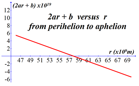
The condition is met over the domain of r. See the graph, right.

Mass of the sun, m₁= 1.988500 x 10³⁰ kg

Universal Gravitational Constant, G = 6.67384 x 10^-11 m³ / kg s²

Lets check the conditions to be met, just to make sure:

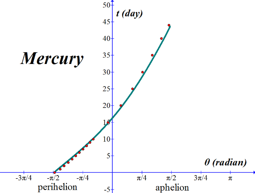
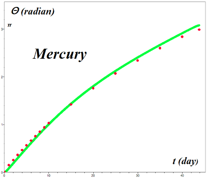
Point series set of data (green) over one-half cycle from previous graph, this time inverted and plotted using Logger-Pro; the Starry Night points (red) are included as well.  The slope of this curve is the angular velocity.  Steepest slope occurs at perihelion, and the slope of the Starry Night point series matches pretty well the slope of this curve.

The green curve here is a graph of equation (21) normalized to t = 0 at perihelion.  Recall that perihelion occurs at θ = -π/2.  We should compare our equations with observational data from Mercury just as a check to make sure that our results are correct; however, I don't have any real data.

 

The next best thing would be to compare our result with someone else's independent calculation - someone whom we trust to produce accurate results.  The red points are taken from the planetary program Starry Night.  Fairly good match, I'd say, so we are on the right track.

---------------------------------------------------------------------------------------------------------------------------------------

(-sqrt(-2.2914E9*(5.54707E10/(1-.2056sin(x)))^2+2.65419E20*(5.54707E10/(1-.2056sin(x)))-7.3615E30)/ 2.2914E9-1.2099E6*asin((-4.5828E9*(5.54707E10/(1-.2056sin(x)))+2.65419E20)/ 5.4541E19))/60/60/24+21.9181

---------------------------------------------------------------------------------------------------------------------------------------

Graph of the same equation over one complete orbit, but phase shifted so that perihelion is at zero angle.

//////////////////////////////////////////////////////////////////////////////////////////////////////////////////////////////////////////////////////////////////////////////////////////////////////////////////////////////////////

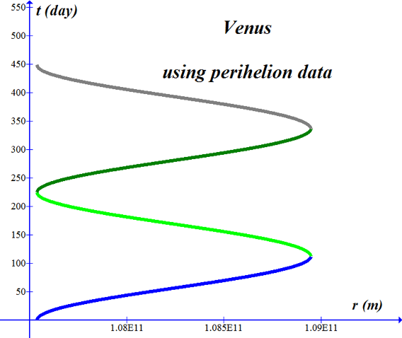
Venus’ orbit is nearly circular. Graphed with an offset so that perihelion occurs at t = 0.

--------------------------------------------------------------------------------------------------------------------------------------------

Equation (blue curve) written for Graph program:

(-sqrt(-1.22603E9*x^2+2.65419E20*x-1.43643E31)/1.22603E9-3.09136E6*asin((-2.45206E9*x+2.65419E20)/1.73050E18))/60/60/24

--------------------------------------------------------------------------------------------------------------------------------------------

///////////////////////////////////////////////////////////////////////////////\\\\\\\\\\\\\\\\\\\\\\\\\\\\\\\\\\\\\\\\\\\\\\\\\\\\\\\\\\\\\\\\\\\\\\\\\\\\\

Venus

 

http://nssdc.gsfc.nasa.gov/planetary/factsheet/venusfact.html

perihelion data                              r_p                                v_p                            P                              m₂

/////////////////////////////////////////////////////////////////////////////////////////////////////////////////////////////////////////////////////////

Mass of the sun, m₁= 1.988500 x 10³⁰ kg

Universal Gravitational Constant, G = 6.67384 x 10^-11 m³ / kg s²

\\\\\\\\\\\\\\\\\\\\\\\\\\\\\\\\\\\\\\\\\\\\\\\\\\\\\\\\\\\\\\\\\\\\\\\\\\\\\\\\\\\\\\\\\\\\\\\\\\\\\\\\\\\\\\\\\\\\\\\\\\\\\\\\\\\\\\\\\\\\\\\\\\

Mars

 

                                                                              http://nssdc.gsfc.nasa.gov/planetary/factsheet/marsfact.html

Mass of the sun, m₁= 1.988500 x 10³⁰ kg

Universal Gravitational Constant, G = 6.67384 x 10^-11 m³ / kg s²

--------------------------------------------------------------------------------------------------------------------------------------------------------------------

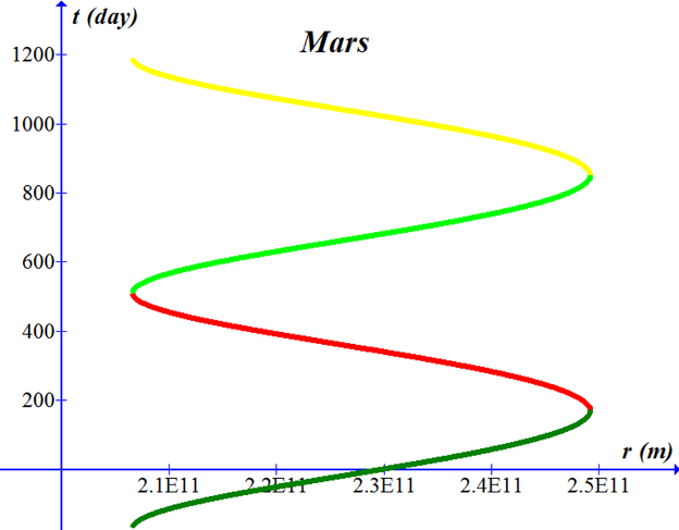
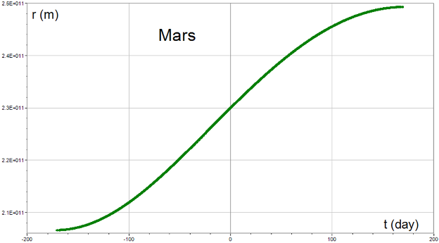
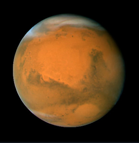
Mars’ time in orbit versus distance from the sun.

 

(-sqrt(-5.82274E8*x^2+2.65419E20*x-2.9982E31)/ 5.82274E8-9.44519E6*asin((-1.16455E9*x+2.65419E20)/ 2.48252E19))/60/60/24

--------------------------------------------------------------------------------------------------------------------------------------------------------------------

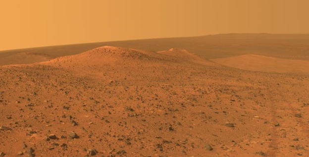
Out for a drive on Mars?

\\\\\\\\\\\\\\\\\\\\\\\\\\\\\\\\\\\\\\\\\\\\\\\\\\\\\\\\\\\\\\\\\\\\\\\\\\\\\\\\\\\\\\\\\\\\\\\\\\\\\\\\\\\\\\\\\\\\\\\\\\\\\\\\\\\\\\\\\\\\\\\\\\\\\\\\\\\\\\\\\\\\\\\

\\\\\\\\\\\\\\\\\\\\\\\\\\\\\\\\\\\\\\\\\\\\\\\\\\\\\\\\\\\\\\\\\\\\\\\\\\\\\\\\\\\\\\\\\\\\\\\\\\\\\\\\\\\\\\\\\\\\\\\\\\\\\\\\\\\\\\\\\\\\\\\\\\\\\\\\\\\\\\\\\\\\\\\\\\\\\\\\\\\\\\\

 

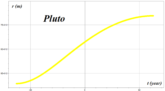
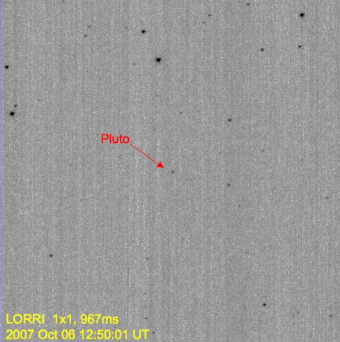
Pluto

 

                                                                              http://nssdc.gsfc.nasa.gov/planetary/factsheet/plutofact.html

aphelion data                             r_a                                v_a                                                P                             m₂

  /////////////////////////////////////////////////////////////////////////////////////////////////////////////////////////////////////////////////////// 

Pluto

7375.93x109 m

3.71x103 m/s

90465 day

0.0131x1024 kg

 

Mass of the sun, m₁= 1.988500 x 10³⁰ kg

Universal Gravitational Constant, G = 6.67384 x 10^-11 m³ / kg s²

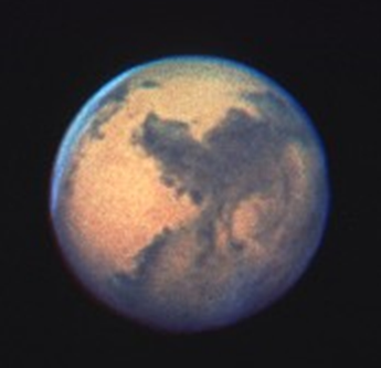
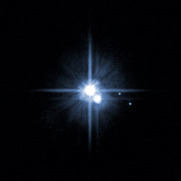
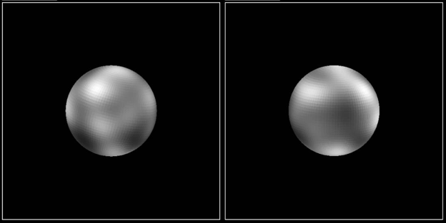
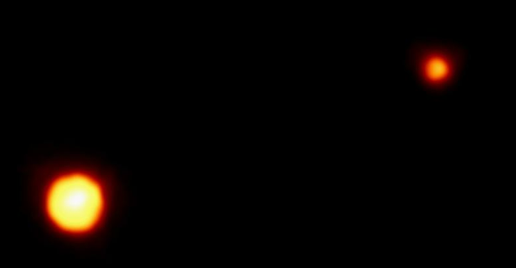
Binary dwarf planet system Pluto and Charon with two moons.

Hubble Telescope, NASA

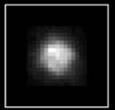
actual images                 

Hubble Telescope Faint Object Camera

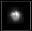
after image processing

///////////////////////////////////////////////////////////////////////////////\\\\\\\\\\\\\\\\\\\\\\\\\\\\\\\\\\\\\\\\\\\\\\\\\\\\\\\\\\\\\\\\\\\\\\\\\\\\\

Pluto and Charon

Venus

aphelion data                                r_a                           v_a                              P                                m₂

   ////////////////////////////////////////////////////////////////////////////////////////////////////////////////////////////////////////////////////////

mnealon@eosc.edu

webpages and Eos image copyright 2015 M  Nealon

Top   Time in Orbit

Page 1   Elliptical Orbits

Page 3   Kepler’s Equation

\\\\\\\\\\\\\\\\\\\\\\\\\\\\\\\\\\\\\\\\\\\\\\\\\\\\\\\\\\\\\\\\\\\\\\\\\\\\\\\\\\\\\\\\\\\\\\\\\\\\\\\\\\\\\\\\\\\\\\\\\\\\\\

so,

Written this way,

and, simplifying, our expression for the time in orbit is

then the expression for r is

therefore,

The integral to solve is

Although we did not show it before, we could easily find the relationship between 𝜅 and the geometric parameters a and b of the ellipse, as follows:

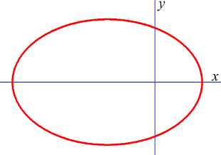
Let’s derive the time versus angle relationship again, with the purpose of writing the equation in a form with ε a bit more conveniently arranged.  If we had the ellipse in a different orientation, as in this figure with the major axis along the x-direction,

we are now ready to look up the integral.

One more step,

The Law of Periods

 

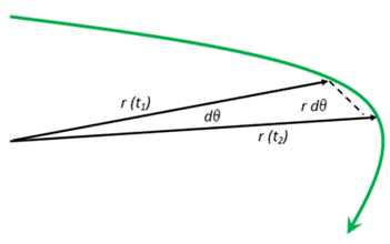
Consider a small area of an ellipse swept out by a planet during a short time, ∆t, as it moves over a small angle, ∆θ.  The lengths of the position vectors which bound the area are not necessarily equal, but close if ∆θ is small.  The area swept out is approximately that given by the area, ∆A, of the triangle.

Written in differential form, this is

Dividing by the time interval, we have

The time rate of change of angle, dθ/dt, has been given earlier in equation (10).  Using that expression, and substituting, we find 

Now using the perihelion expression for L, we have

which is the areal velocity and is a constant throughout the orbit.  For one complete orbit, the period is

or,

Now we need to know the area of the ellipse.  An ellipse may be characterized by two quantities, so let us eschew as best we can the purely geometric terms in describing the ellipse and use astronomical properties which are measurable: the orbital period and the perihelion distance.  We may also use the eccentricity. 

 

In geometry texts the semi-major axis typically is called a, and the distance from the focal point to the center of the ellipse is c = ε/a.  Using these, then, we can write

or, r_p in terms of a,

We also have

These two relationships imply that

and we all know that

The semi-minor axis, b, is usually written as

which becomes

The area is given by

With substitution, this becomes

After substituting in for r_p we have

Kepler again.

The period, then, is

Perfect, except that now we need an expression for v_p.  Where else would we look other than the well-used work-energy theorem?  The unnumbered equation just above equation (18) gives us the result we need.

Now we may simplify the expression for the period.  The algebra is much easier to deal with if we square both sides

For Mercury; calculate in days.

 

τ = 87.969 day = 7.6005x10⁶ s

ε = .2058

r_p = 46.00x10⁹ m

v_p = 58.98x10³ m/s

G = 6.67384 x 10^-11 m³ / kg s²

M  ̴  mass of the sun, m₁= 1.988500 x 10³⁰ kg.

Revisit Time as a Function of Angle

 

Just above we wrote the differential area,

Writing the indefinite integral of both sides gives us

Regarding the indefinite nature of the integration: on the right-hand-side we can always use a phase shift to orient the ellipse after the integration;  the integral on the left-hand-side can be dealt with easily enough, as follows: at some time t = 0, we let θ = 0; furthermore, we know that the areal velocity, that is, the rate at which area is swept out by the planet, is a constant.  This means that the area subtended by the angle θ up to a time t is a fraction of the total area πab.  We can then write

With this, then, we have

We have already written the expression for r in terms of θ,

where

and the area,

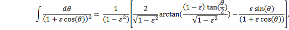
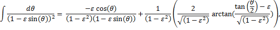
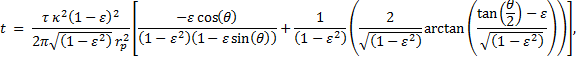
Bringing these together we find yet another integral to solve giving us the time in orbit as a function of angle,

This one we shall look up.  [Tables of Integrals and Other Mathematical Data, H. B. Dwight, 4^th ed., Macmillan Publishing Co., 1961.]

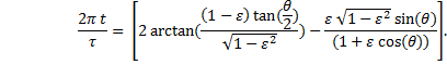
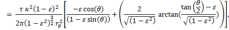
under the condition that 1 > ε², which it is.  So,

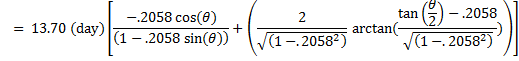
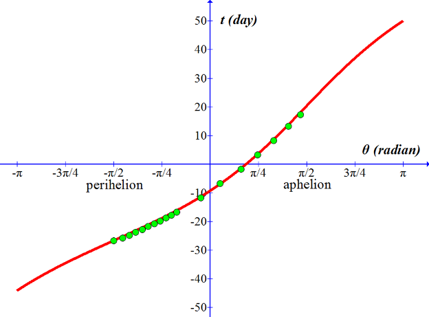
Graph of equation (22), time as a function of angle, in red.  Unlike the previous version of t(θ), this covers the entire orbit as a continuous function.  Starry Night values (green) plotted just as a check.

 

--------------------------------------------------------------------------------------------

13.70 ((-.2056cos(x)/(1-.2056sin(x)))+2.044atan((tan(x/2)-.2056)/.9786))

---------------------------------------------------------------------------------------------

therefore,

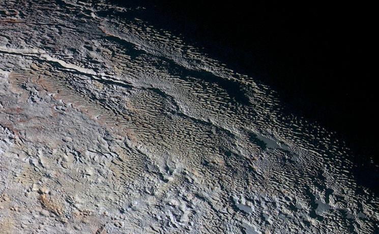
“Rounded and textured mountains rise up along Pluto's day-night terminator and show intricate patterns of blue-gray ridges and reddish material in between. This view, roughly 330 miles across, combines blue, red and infrared images taken by the Ralph/Multispectral Visual Imaging Camera (MVIC) on July 14, 2015, and resolves details and colors on scales as small as 0.8 miles.  Taken by NASA's New Horizons.”

from NASA