|
Page 1 Elliptical Orbits |
|
Page 2 Time Dependency |
|
Page 3 Kepler’s Equation |
|
Elliptical Planetary Orbits Derived from Newtonian Mechanics |
|
The notion that planets revolve about the sun in elliptical orbits was found empirically by Johannes Kepler during his little “war with Mars.” Later, the fundamental principles elucidated by Isaac Newton provided a firm theoretical basis for understanding such orbits. Newton’s principles can produce quite general solutions to this idealized two-body problem of course, showing that planets may follow any of a number of trajectories described by conic sections. Of interest here, however, is only in showing that an expression for one particular orbit - the ellipse - falls right out of the mathematics.
In general, a straightforward technique for deriving an object’s trajectory is to begin with Newton’s second law of motion, F = ma. Substituting an expression for the force into the left-hand-side and writing the acceleration as the second time derivative of position results in a set of equations which can be integrated in order to find the object’s position as a function of time. Integrating twice may be a bit difficult for some trajectories.
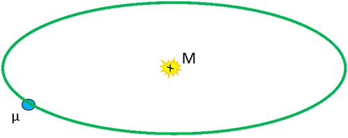
Since the time dependence is not really the desired solution at the moment, the problem can be simplified by removing any time dependency and solving for the planet’s path in ordinary two-dimensional space. This solution displays the elliptical nature of the orbit. Properly speaking, though, for a planet with a moon or moons, it is the center-of-mass, or, barycenter of the planet/moon system which traces the elliptical orbit about the sun.
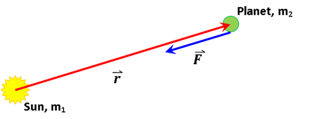
Newton’s expression for the gravitational force, F, is written in terms of the planet’s radial position, r: |
|
where m1 is the mass of the sun, m2 is the mass of the planet, r is the radial distance between the sun and planet, G is the universal gravitational constant, is the unit vector in the radial direction.
The radial vector is |
|
and the force can be written explicitly as a function of r, |
|
Note that the unit vector in the radial direction is |
|
Note on Center of Mass of Sun/Planet System
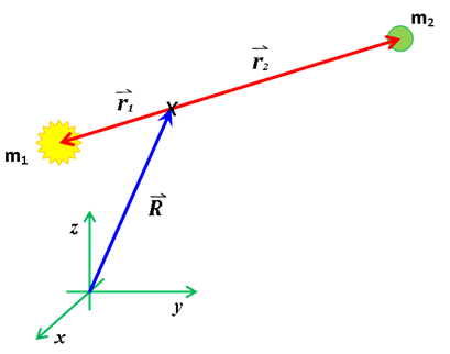
If the origin of our coordinate system is as shown in this figure: |
|
then the kinetic energy of the system, KE, is the sum of the kinetic energy of motion of the center of mass plus the kinetic energy about the center of mass, given as |
|
where R is the position vector of the center of mass and r1 and r2 describe the positions of the bodies relative to the center of mass. We have employed the dot notation for the first derivative with respect to time. These two position vectors are related as |
|
If the origin of our coordinate system is at the center of the sun as described above in the first figure, then solving for the motion of the planet presumes that the sun is fixed in place; that is, as though there were no rotation of both bodies about a common center of mass. This implies that the sun has no kinetic energy within the solar system. This may be approximately true in our solar system, where the largest planet is small (but not necessarily insignificant considering modern astronomical measurement techniques) compared to the sun.
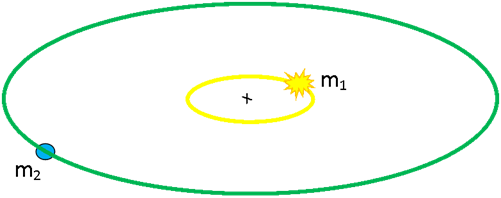
If instead we wish to place the origin at the center of mass of the Sun/Planet system, we would write the position vectors as |
|
and |
|
With these, the kinetic energy about the center of mass can be reduced to |
|
Since we have no interest here in the motion of the solar system within the galaxy we may ignore altogether R and its time derivative. This process of ignoration is simply a matter of dropping the first term in the expression for kinetic energy.
Thus the system is reduced to an equivalent one-body problem where the planet acts as though it has an effective, or “reduced” mass |
|
and the sun acts as though it is a body of mass |
|
Newton’s universal law of gravitational attraction for a body of mass M and a body of mass μ results in the same force as given above. This equivalent one body problem is as though there were a single mass, M, at the center of rotation and a body of mass μ in orbit. |
|
In our solar system, we may wish to ignore the reduced mass if we consider the planetary masses small compared to the sun's mass. For example, the mass of Jupiter is 1898.3x1024 kg and the sun’s mass is 1.9855x1030 kg. For this system, the reduced mass is 1893.2x1024 kg: a reduction of about 0.3%, and M = 1.9874x1030 kg; so we can see here that using the reduced mass in the solar system is not really necessary.
There are other systems in which the two masses are comparable, such as binary star or planet/moon orbits. The analysis presented here is general and can be applied to these systems. For our purpose we will use terminology of the sun/planet system: aphelion and perihelion, but the general terms are apoapsis and periapsis. |
|
Two-dimensional nature of the orbit
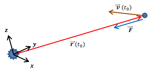
That the orbital path of a planet about the sun is two-dimensional has been asserted without any proof. This assertion should be shown to be true, perhaps, before moving on to the derivation of elliptical orbits. This two-dimensional nature of the orbits can be understood with a physical argument, as follows: the gravitational force vector is always anti-parallel to the position vector; at any given moment the planet’s position vector and velocity vector form a plane (except in the particular case of free-fall in which they are co-linear). Since the force vector is also in this plane there is no component of force perpendicular to the plane, and thus, there is no force to drive the planet outside the plane. This is a consequence of the centripetal (“center-directed”) nature of the gravitational force.
The idea of planar orbits can easily be shown mathematically. Define the moment which was just described as occurring at time t0, and arrange the coordinate system such that the x-y plane aligns with the r-v plane. Since the component of force in the z-direction is zero, we can write this component in terms of acceleration, az, as |
|
Dividing through by the mass of the planet and writing an indefinite integral over time, we obtain |
|
This constant of integration is the z-component of speed at time t0, which is zero at t = t0 because at that moment the velocity vector is in the x-y plane; we are therefore left with vz(t) = 0. Now we integrate a second time, |
|
Here, the constant of integration is z(t0) = 0. This result means that the time dependency of the z-component of position is zero; in other words, since the planet is in the plane z = 0 at some moment t0, then it must always be in that plane.
Yet another way to prove the assertion of two-dimensional motion is to take a look at the time derivative of the cross product of position with momentum. The momentum, p, of the planet is defined as the planet’s mass times its velocity. The reason for taking the derivative will be clear in a moment. Using vector notation, |
|
Notice that the first term on the right hand side is |
|
since the cross product of a vector with itself is zero. Also, recall that the gravitational force vector and the position vector are anti-parallel. The cross product of any two co-linear vectors is zero; therefore |
|
so, |
|
Substituting these into (4), we have |
|
Now, taking an indefinite time integral of both sides results in a constant of integration, |
|
This means that if r and v are in a plane at some moment and then at some later time one of them (or the other or both) deviates from that plane – then their cross product would point in a different direction and thus not be a constant. Therefore r and v are restricted to one plane, and the two-dimensional nature of the orbit is proven.
Perhaps it seems as though equation four was written as if the end of the proof and the direction towards it were already known. They were, of course, but it does not make the proof any less rigorous. This seemingly post res nature of some mathematical proofs will appear again later.
The linear momentum of the planet is |
|
Angular momentum, , is the cross product of position with linear momentum, so from equation (5) the angular momentum must be constant |
|
Incidentally, since the angular momentum is a constant throughout the orbit, we could evaluate it at any point. At both perihelion, the point of closest approach to the sun, and aphelion, the furthest point in the orbit, the planet’s position vector is perpendicular to the velocity vector. Let rp be the perihelion distance and vp the velocity at perihelion, and let ra be the aphelion distance and va the velocity at aphelion; the magnitude of angular momentum, then, is |
|
Attempt at a perspective rendering of the x-y plane drawn co-planer with the r-v plane at time t0. It is not necessary that either the x- or y-axis align with F, v, or indeed, r. |
|
Polar coordinate diversion
Since the problem has been reduced to two-dimensions, and the force is centripetal, it would seem to be ideal to operate in polar coordinates (cylindrical coordinates, really, if ever we invoke the z-direction).
At this point it may be a useful diversion to step explicitly through the conversion between coordinate systems. Let θ be the angle between the position vector and the x-axis. We now have |
|
The position vector is |
|
so the unit vector in the direction of the position of the planet is |
|
where the usual unit vector notations i and j in the x-y coordinate system are used. Therefore, the radial vector is written as |
|
The dot notation for time derivative is employed here. Likewise, we have |
|
and |
|
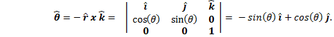
Since the unit vector in the direction of increasing angle θ is in the x-y plane and is perpendicular to , it can be found from the negative (to give it the correct direction) of the cross product between and the unit vector in the z-direction, . |
|
If required, these last two equations could be rearranged to give i and j in terms of |
|
We may consider the two unit vectors in polar coordinates, , as moving along with the planet. This means that their direction is time dependent. Let’s take a look at the time derivative of the position unit vector. |
|
Velocity
Now let’s use these polar coordinates to discuss the velocity of the planet before we return to the subject of angular momentum. The velocity of the planet is the time derivative of the position vector, namely, |
|
[Or, equally, the time derivative in rectangular coordinates may be taken first, and then the complete conversion to polar coordinates is made: |
|
Now substituting in the unit vectors we have |
|
and with a little algebra the same result obtains.] |
|
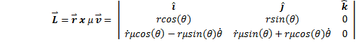
Angular Momentum
We know from equation (6) that the angular momentum is constant, so why not calculate the cross product? We have the position vector, equation (7), and we can use the velocity vector as expressed in equation (9). |
|
Remove the dot notation and write the magnitude of the angular momentum as |
|
By the way, dθ/dt = ω, is the planet’s angular velocity. Rearrange the expression for angular momentum to find |
|
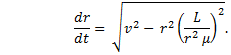
Now use equation (8) to write an expression for the magnitude of the velocity, again removing the dot notation: |
|
Solve this for dr/dt, and substitute equation (10) in for dθ/dt: |
|
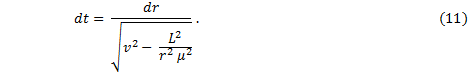
Now, solve for dt |
|
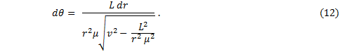
In order to show that the orbit is an ellipse, the time dependency of this equation needs to be removed and the equation should be written in terms of the angle. Use equation (10) once again; solve it for dt and substitute that into (11), thusly: |
|
or, |
|
or, |
|
Integration
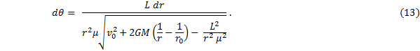
Substitute that last expression into equation (12). |
|
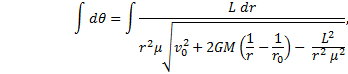
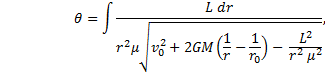
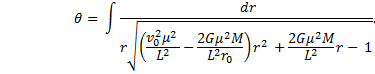
Now to find the position as a function of angle it is necessary to integrate both sides of equation (13). An indefinite integral will give the general result. |
|
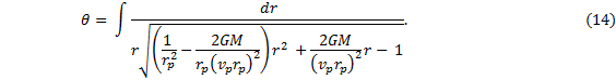
At this juncture it might be helpful to simplify the appearance of this equation by using the expression given above for angular momentum evaluated at either perihelion or aphelion. If we choose perihelion, say, then let r0 = rp and v0 = vp. We then have |
|
This integral is of the form |
|
and |
|
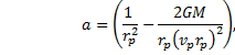
where |
|
and |
|
Calculus diversion
A table of integrals would be handy in finding the solution to that integral. However, seeing this integration performed might prove instructive. Start with the trigonometric function cosine. Let x = cos(θ). A similar solution could be found if we were to begin with the sine function; at any rate, let's take the derivative of cosine with respect to θ. |
|
or, |
|
Now, notice that |
|
and take the arcsine of both sides; |
|
Here we take the derivative of both sides with respect to θ |
|
Now, substitute x for cos(θ) and substitute equation (15) for dθ. |
|
Using a trigonometric identity and again reverting to the variable x, we have |
|
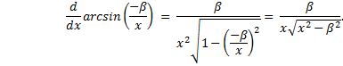
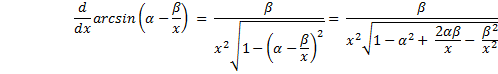
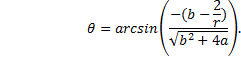
That’s the derivative of the arcsine. Let’s try a different argument in the arcsine — an inverse function — and include an arbitrary constant, - β; the chain rule for derivatives gives us |
|
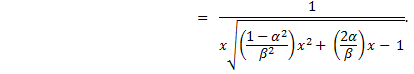
This is not quite the result we are after – but close. We can find what we need by using a slightly more complex argument in the arcsine function, and again using the chain rule. |
|
Written in the form we recognize, this becomes |
|
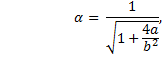
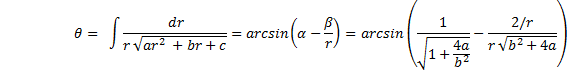
Integrate to obtain the final result |
|
There we have it. |
|
where |
|
and |
|
The Solution
The solution to equation (14) is now clear. |
|
The condition which makes this solution possible is that the argument in the arcsine function must be between -1 and 1. This occurs if the numerator is less than the denominator: |
|
Another solution to equation (14) is |
|
This requirement is that |
|
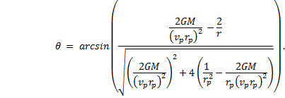
Now let us write the solution in terms of the orbit parameters. We will use the perihelion. |
|
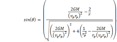
Now take the sine of both sides and solve for r. |
|
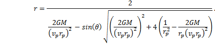
Therefore, |
|
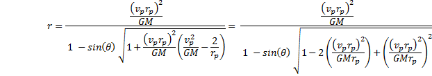
Simplifying, this becomes |
|
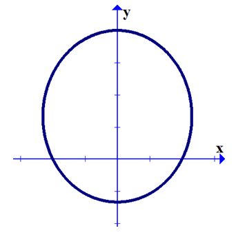
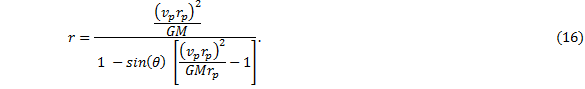
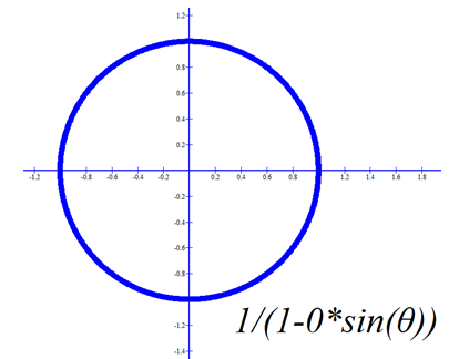
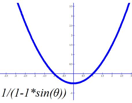
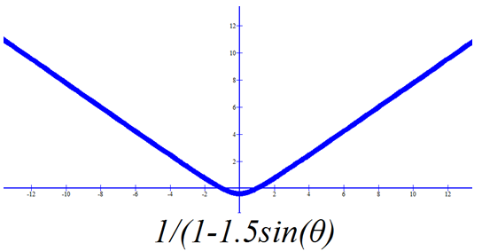
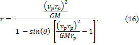
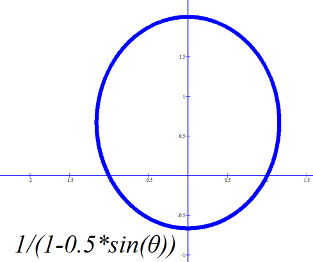
This is the equation which describes in polar coordinates the orbit as a conic section. The other solution to equation (14) produces a plus sign instead of a negative sign in the denominator (the one in front of the sine function). This puts the sun at the other focal point in the case of elliptical or hyperbolic orbits and opens the parabolic orbit in the opposite direction, but the overall shape of the curve would be unaltered. Both solutions, however, place the major axis of the curve along the y-axis. For the elliptical solution, this figure illustrates the general shape as written in equation (16): |
|
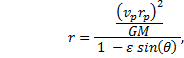
The expression inside the square bracket is the eccentricity, ε, of the orbit. Rewriting, we have |
|
where |
|
Phase of the Ellipse
An inspection of the figure shows that the phase of the ellipse may at first seem a bit odd: perihelion occurs at θ = - π/2. Notice that if θ = 0 then the distance along the x-axis from the origin to the curve is given by |
|
As mentioned above, there is a solution which might be found when starting with the cosine function. This can produce two expressions for r; one with (1 + ε cos(θ)), and one with (1 - ε cos(θ)) in the denominator. These solutions have the major axis aligned with the x-axis.
This cosine solution places either the aphelion or perihelion at θ = 0, which might be preferable, for exampe, when graphing the solution. However, a simple phase shift in the trig functions after finding the solution will accomplish the same rotation of the ellipse.
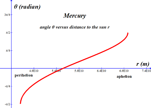
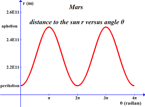
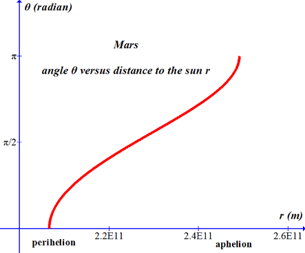
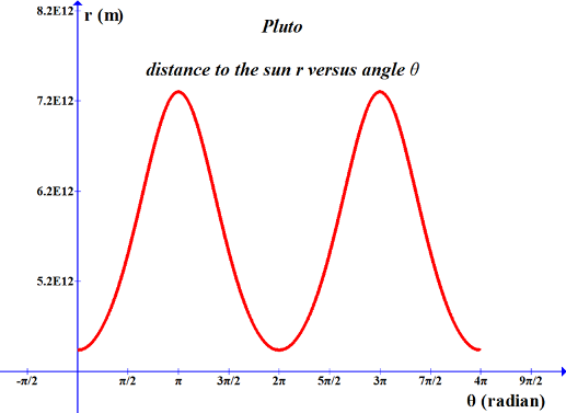
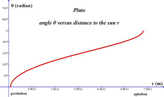
We might as well graph the expression for the distance to the sun versus angle just to see what it looks like. Here is the graph for Mercury, Mars, and Pluto over two cycles. Also, while we are at it, let’s look at θ versus r from perihelion to aphelion – over an angular difference of π. Note the asymmetry in both curves. This asymmetry indicates that the planet’s speed is not constant throughout its orbit. These graphs were made using the mass m1 rather than M since the masses of these planets are so small compared with the sun. Also, the graphs of Mars and Pluto have been phase shifted to place the perihelion at θ = 0. |

|
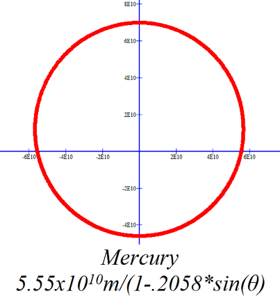
-------------------------------------------------------------------------------------------------------------------------------- Mercury; r versus θ, Equation (16) Function written in the form for Graph program: 5.5466E10/(1-.2056sin(x)) -------------------------------------------------------------------------------------------------------------------------------- |
|
-------------------------------------------------------------------------------------------------------------------------------- Mercury; θ versus r Function written in the form for Graph program: asin((3.6058E-11-(2/x))/7.4203E-12) -------------------------------------------------------------------------------------------------------------------------------- |
|
-------------------------------------------------------------------------------------------------------------------------------- Mars; r versus θ, Equation (16) Function written in the form for Graph program: 2.2591E11/(1-.09336sin(x+4.7135)) --------------------------------------------------------------------------------------------------------------------------- |
|
-------------------------------------------------------------------------------------------------------------------------------- Mars; θ versus r Function written in the form for Graph program: asin((8.8531E-12-(2/x))/8.26516E-13)+1.5708 -------------------------------------------------------------------------------------------------------------------------------- |
|
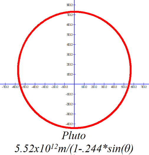
-------------------------------------------------------------------------------------------------------------------------------- Pluto; r versus θ, Equation (16) Function written in the form for Graph program: 5.519E12/(1-.244sin(x+4.7135)) -------------------------------------------------------------------------------------------------------------------------------- |
|
-------------------------------------------------------------------------------------------------------------------------------- Pluto; θ versus r Function written in the form for Graph program: asin((3.6235E-13-(2/x))/8.8423E-14)+1.5708 -------------------------------------------------------------------------------------------------------------------------------- |
|
webpages and Eos image copyright 2015 M Nealon |
|
Orbital Types |
|
Planetary Orbits
Let’s look up the perihelion distances and speeds of the planets and calculate the eccentricity. The perihelion and aphelion values found on NASA webpages are listed in the table below. NASA’s eccentricities are not measured values, but are calculated from orbital parameters.
Mass of the sun, m1= 1.988500 x 1030 kg (http://nssdc.gsfc.nasa.gov/planetary/factsheet/sunfact.html)
Universal Gravitational Constant, G = 6.67384 x 10⁻¹¹ m3 / kg s2 (http://nssdc.gsfc.nasa.gov/planetary/factsheet/fact_notes.html [see also the note at the top of this NASA webpage for the sources of their information]) |
|
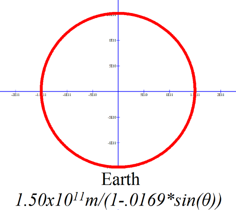
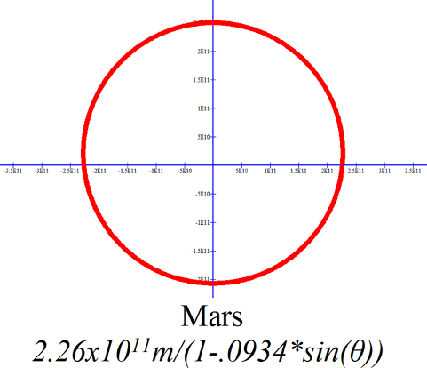
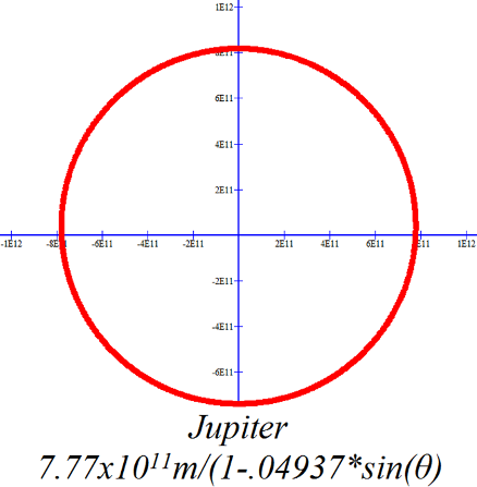
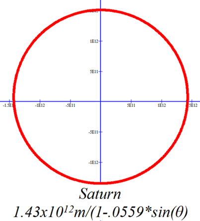
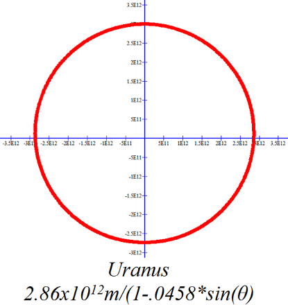
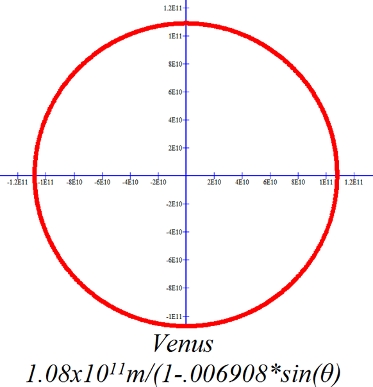
Graphs of Planetary Orbits, Equation (16)
On the scales of these graphs only Mercury, Pluto and perhaps Mars have readily obvious elliptical orbits. The elliptical nature of the other orbits is a bit more subtle. |

|
Top Elliptical Orbits |
|
Page 2 Time Dependency |
|
Page 3 Kepler’s Equation |
|
Using the Work-Energy Theorem
Equation (12) is the starting point in finding the shape of the orbit, and so we need an expression for the velocity, v. The v2 term makes us think of the kinetic energy of the planet, so we might look at the work-energy theorem to aid us in finding the solution. Let us say that the planet has some velocity v0 at some distance r0 and moves to some other (variable) position along its orbit and has a speed v and variable position r.
The work done by the gravitational force in moving the planet from one position to another is equal to the change in the planet’s kinetic energy. If the planet moves closer to the sun then the work done by the gravitational force is positive and the change in kinetic energy is also positive. If the planet moves further away from the sun then the work done by the gravitational force is negative and the change in kinetic energy is also negative. Either case gives us the same expression for v. |
|
where M = m1 + m2; so the integral becomes |
|
Using this and solving the work-energy theorem for v2 we have |
|
Note: The initial conditions r0 and v0 may occur at any place one may choose along the orbit, but typically these are evaluated at either the aphelion or perihelion. At those places the position vector and velocity vectors are at right angles to each other. Since aphelion, ra is the furthest distance from the sun, it is always greater than r, and the difference (1/r – 1/ra) is always positive. However, since perihelion is the point of closest approach, the difference (1/r – 1/rp) is always negative. This is of no consequence now, but later we must choose perihelion or aphelion carefully in order that the argument of an arcsine function is never greater than 1 or less than -1. |
|
recalling that and are parallel, so there is no need, really, for the dot product. Tackle the integral first. Write the magnitude of the force as |

|
Notes on Eccentricity This eccentricity is an interesting result:
1. Notice that if we had chosen the aphelion as our initial condition, then the result would be, well, not exactly the same, but similar: |
|
2. Let us look at the results of the work energy theorem again. Using the perihelion as initial condition we have |
|
Now then, if the planet just happens to be at aphelion, we would let r = ra, and, correspondlingly set v = va, then |
|
We also know, based on the idea of conservation of angular momentum, that (vp rp)2 = (va ra)2. We could substitute at will either of these into the expression for eccentricity if we like. Instead, however, let’s rewrite that expression and substitute for va 2. |
|
Further manipulation gives us |
|
and now, |
|
Simplifying, we have |
|
Subtract one from both sides and simplify to obtain the expression for ε. |
|
Naturally, the aphelion expression for ε produces the same result. |
|
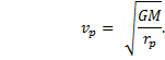
The eccentricity is zero if ra = rp, or, if |
|
This is the orbital speed of a planet in uniform circular motion. Since the orbital speed is constant, we can write the speed as vp = v. In other words, the orbit is a circle with radius |
|
The orbital period, τ, is given by the circumference of the orbit divided by the linear velocity. |
|
or, |
|
Circular
If ε = 0. |
|
Kepler. |
|
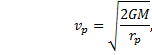
Parabolic
If ε = 1.
The eccentricity is 1 if |
|
or, |
|
and the orbit is parabolic. The velocity is exactly that of “escape”, so the body in orbit should never return; however, a slight perterbation of the orbit may cause the body to be captured. [The escape velocity refered to here is not the velocity of escape from the surface of the sun, but the escape velocity at the point of closest approach.] |

|
Hyperbolic
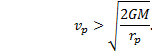
If ε > 1.
The eccentricity is greater than 1 if the velocity of closest approach is greater than the corresponding escape velocity: |
|
In this case the orbit is hyperbolic. The body will not return. |
|
and the orbit is an ellipse with the sun at one of the focal points. |
|
Elliptical
If 0 < ε < 1.
If the eccentricity is between zero and 1, then |

|
|
Perihelion distance (x109 m)* |
Perihelion velocity (x103 m/s)* |
Aphelion distance (x109 m)* |
Aphelion velocity (x103 m/s)* |
Eccentricity Calculated from (18) |
Mass (x1024 kg)* |
|
Mercury |
46.00 |
58.98 |
69.82 |
38.86 |
0.2058 |
0.3301 |
|
Venus |
107.48 |
35.26 |
108.94 |
34.79 |
0.006908 |
4.8676 |
|
Earth |
147.09 |
30.29 |
152.10 |
29.29 |
0.01690 |
5.9726 |
|
Mars |
206.62 |
26.50 |
249.23 |
21.97 |
0.09336 |
0.64174 |
|
Jupiter |
740.52 |
13.72 |
816.62 |
12.44 |
0.04937 |
1898.3 |
|
Saturn |
1352.55 |
10.18 |
1514.50 |
9.09 |
0.05590 |
568.36 |
|
Uranus |
2741.30 |
7.11 |
3003.62 |
6.49 |
0.0458 |
86.816 |
|
Neptune |
4444.45 |
5.50 |
4545.67 |
5.37 |
0.0130 |
102.42 |
|
Pluto** |
4436.82 |
6.10 |
7375.93 |
3.71 |
0.244 |
0.0131 |
|
|
|
|
|
|
|
|