|
Page 1 Elliptical Orbits |
|
Page 2 Time Dependency |
|
Page 3 Kepler’s Equation |
|
Kepler’s Equation |
|
This formula, derived at the bottom of the previous page, is called Kepler’s equation. The planet’s time-in-orbit, t, is given as a function of its angular position, θ. Kepler’s idea to solve the equation for the angular position as a function of time (despite the transcendental nature of the problem) was to use the area swept out by the planet as a proxy for a clock. This is possible since, as indeed Kepler was first to observe, the areal velocity is a constant throughout the orbit.
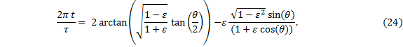
In order to accomplish this same task let us begin with the x- and y-coordinates of the planet’s position, P, along the ellipse. The origin of our x-y coordinate system is at the sun, and the distance from the sun to center of the ellipse is aε. In Cartesian coordinates an ellipse with this off-set and with semi-major axis a and semi-minor axis b is given by |
|
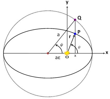
Next, if we escribe a circle of radius b inside the ellipse and project the planet’s position parallel to the x-axis to a point Q’ onto this new circle, as shown below, then the line drawn from Q’ to the center of the ellipse makes the same angle ψ with respect to the x-axis. (We leave this assertion as an exercise for the reader to prove.) |
|
We can see these relationships geometrically, as follows: Kepler inscribed a circle around the ellipse with the radius a, and projected the position of the planet perpendicular to the x-axis onto the circle, point Q in this figure. The parameter ψ is a measure of the angle between the x-axis and the line from the center of the ellipse to Q. From the figure we see that x is related to the cosine of the angle ψ by |
|
so we know right away that we could characterize the ellipse with a parameter ψ, where |
|
From this figure, we have the y-coordinate, |
|
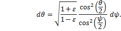
What we want is the relationship between ψ and θ. Recall that (somewhere or other) we had |
|
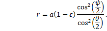
These two equations give us r as a function of ψ, |
|
so we can write the magnitude of the position vector as |
|
or, as we prefer for now |
|
Add εr to both sides of equation (26), and recalling that (1-ε2) = (1-ε)(1+ε), we have |
|
Now we can substitute in the ψ dependence of r from equation (25) into the right-hand-side only and rearrange: |
|
Subtract εr from both sides of equation (26), and simplify in a similar manner to obtain |
|
Divide equation (27) by (26); this leads to |
|
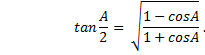
At this point we can use the half-angle formula for the tangent function, which in general is |
|
With this, then, we now have |
|
Solve this last for ψ: |
|
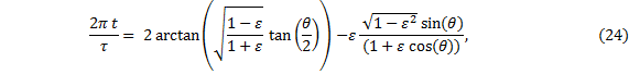
This equation gives us the angular position of the planet as measured from the center of the ellipse, given any angular position θ as measured from the sun. This happens to be the first term on the right-hand-side of Kepler’s equation (24).
At this juncture we wish to put Kepler’s equation into the standard form found in all the texts. In order to do so, we could either re-derive Kepler’s equation with this variable change from θ to ψ using integral calculus, or we could simply transform the rest of Kepler’s equation (24) as already written using algebra only. We shall do both, just for the exercise. |

|
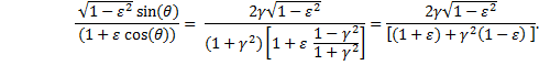
The fraction in the second term of Kepler’s equation is |
|
A) Transform Kepler’s Equation in Variable θ into Variable ψ
In order to transform the second term on the right-hand-side of Kepler’s equation (24) [we have transformed the first term already], we begin by solving equation (29) for θ and taking the sine and cosine of θ . Let us introduce the momentarily useful symbol γ. |
|
We now have |
|
and consequently, |
|
where we have used the double-angle formulæ for the sine and cosine functions, which are, in general, |

|
Now substitute in the expression for γ |
|
Therefore, Kepler’s equation becomes |
|
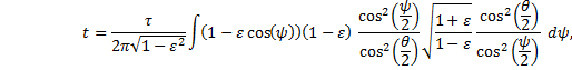
B) Derive Kepler’s Equation by Integration Using Variable ψ
Since we are going to use this equation, (23) from the previous page (substituting in for b), |
|
or, |
|
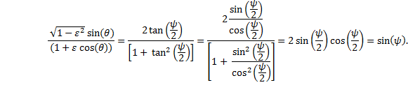
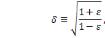
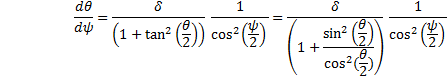
we will need the differential dθ. Begin by solving equation (29) for θ and using, temporarily, the symbol δ. If |
|
and we have this one, equation (27), rearranged and having had the half-angle formula applied to the cosines: |
|
since the secant is the inverse of the cosine. Substituting the original variable, θ, back into the solution may seem odd, but it removes the δ in the denominator and in just a moment we will cancel it anyway: |
|
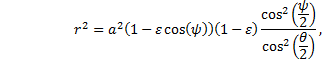
The integral we’re after solving includes an r2 term, so we will find two separate expressions for r and multiply them together. We have this one, equation (25): |
|
Therefore, |
|
then |
|
Now, |

|
A) Series Expansion
For Kepler’s equation in this form |
|
How to Use Kepler’s Equation
Solutions to Kepler’s equation give the planet’s angular position, either θ or ψ, as a function of time. From that, then, the radial distance, r, as a function of time may be calculated with equation (25) or (25’). For a parametric representation in (r, θ) of the orbit in polar coordinates, time may be used as the parameter. The degree to which any of these approximate solutions are either appropriate or sufficiently accurate for any particular application is left as a decision for the reader. As always, an appeal to nature is warranted.
This is a look at several techniques for finding a solution to the equation: |
|
and the integral is |
|
which is, after simplifying, |
|
Thus, upon integrating and rearranging, we have again Kepler’s equation in the standard form, |
|
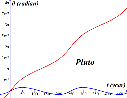
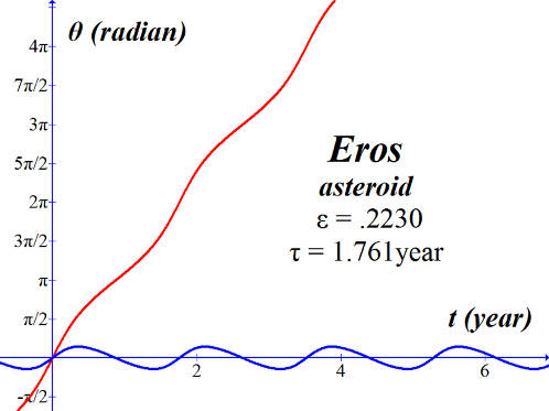
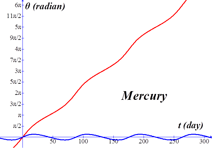
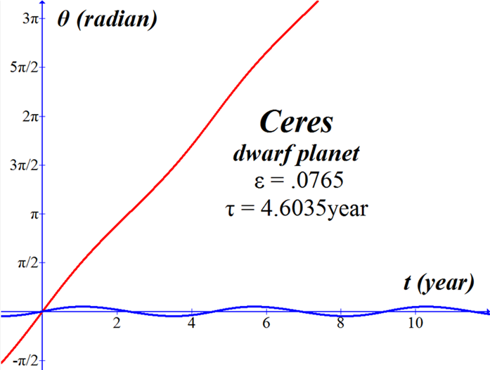
This function is plotted below in red for Mercury, Pluto, the asteroid Eros, and the dwarf planet Ceres. The blue curves are plots of θ(t) with all terms except the linear first term (2πt/τ); these blue curves are included in the graphs simply to illustrate the asymmetric oscillatory nature of the function a bit more clearly. |
|
this series expansion in θ works for planetary orbits if terms in ε3 are included, but still-and-all it works best for small ε. Without derivation, we have |
|
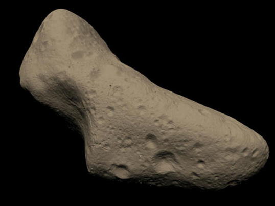
“Reconstructed” image from NASA
Eros Fact Sheet http://nssdc.gsfc.nasa.gov/planetary/text/eros.txt
///////////////////////////////////////////////////////////////////////////////\\\\\\\\\\\\\\\\\\\\\\\\\\\\\\\\\\\\\\\\\\\\\\\\\\\\\\\\\\\\\\\\\\\\\\\\\\\\\\\ |
|
----------------------------------------------------------------------------------------------------------------------------- (2*pi*x/tau)+2*epsilon*sin(2*pi*x/tau)+(5*(epsilon^2)/4)*sin(4*pi*x/tau) +((epsilon^3)/12)*(13*sin(6*pi*x/tau)-3*sin(2*pi*x/tau)) tau = 87.969 earth day epsilon = .2056
“Graph” program. ----------------------------------------------------------------------------------------------------------------------------- |
|
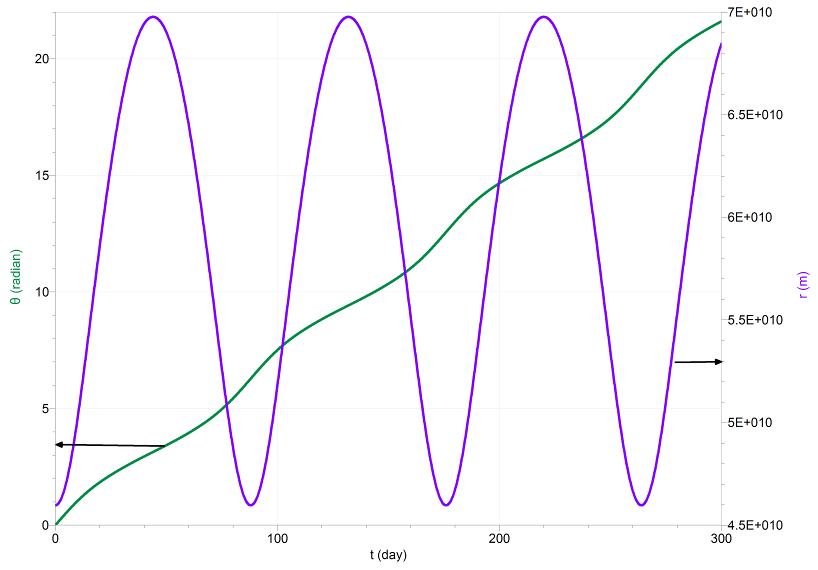
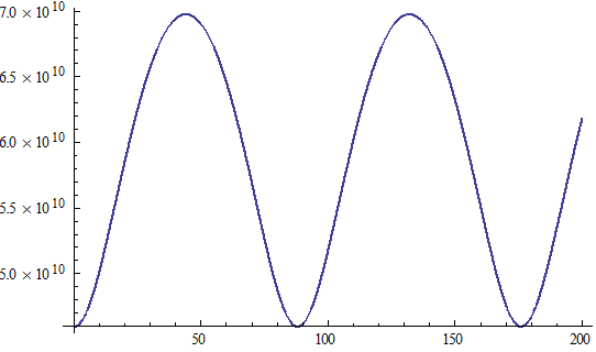
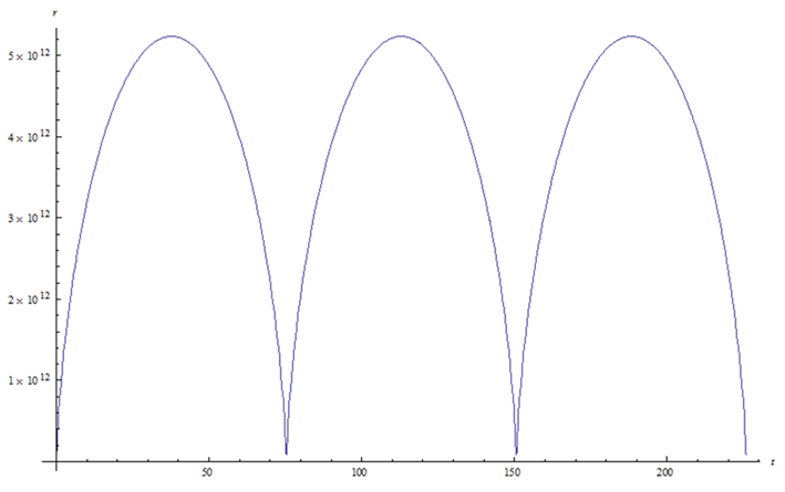
Graph of θ versus t over a few orbits for Mercury (in green, left axis) and a graph of r versus t (violet, right axis) using |
|
where a = 5.787x10¹⁰ m.
“Logger-Pro” program. |
|
Parametric representation of Mercury’s orbit in r and θ as calculated above using Series Expansion.
//////////////////////////////////////////////////////////////////////\\\\\\\\\\\\\\\\\\\\\\\\\\\\\\\\\\\\\\\\\\\\\\\\\\\\\\\\\\\\\\\\\\\\\\ |
|
Mercury |
|
Mercury |
|
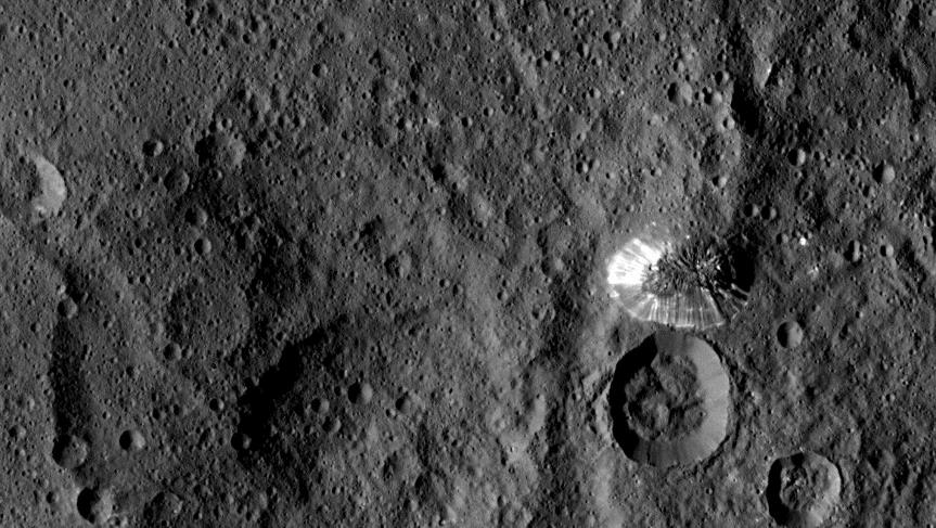
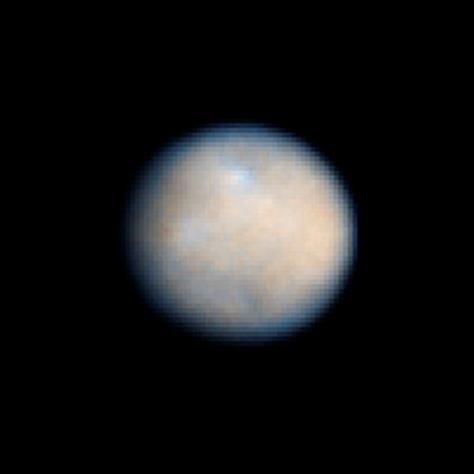
Streaked Conical Mountain on Ceres Captured by Dawn Spacecraft, NASA |
|
Ceres, Keck Observatory |
|
Ceres, NASA, Hubble Telescope |
|
/////////////////////////////////////////////////////////////////////////////////////////////////////////////////////\\\\\\\\\\\\\\\\\\\\\\\\\\\\\\\\\\\\\\\\\\\\\\\\\\\\\\\\\\\\\\\\\\\\\\\\\\\\\\\\\\\\\\\\\\\\\\\\\\\\\\\\\\\\\\\\\\\\\ |

|
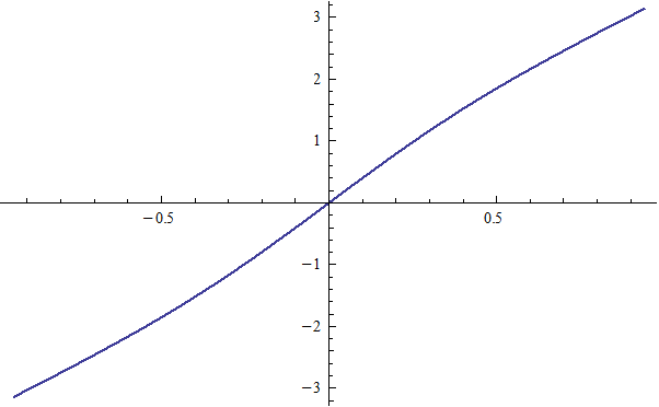
The red curve is the series expansion in θ for Pluto. The blue curve is a plot of θ(t) with all terms except the linear first term, 2πt/τ.
//////////////////////////////////////////////////////////////////////\\\\\\\\\\\\\\\\\\\\\\\\\\\\\\\\\\\\\\\\\\\\\\\\\\\\\\\\\\\\\\\\\\\\\\ |
|
Series expansion in θ for Eros the asteroid. |
|
B) Bessel’s function
According to Encyclopæda Britannica, Bessel’s functions were “. . . derived around 1817 by the German astronomer Friedrich Wilhelm Bessel during an investigation of solutions of one of Kepler’s equations of planetary motion.” Let’s begin with Kepler’s equation in this form: |
|
to answer the following questions: |
|
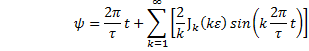
The solution can be found using the sum of Bessel’s functions of the first kind, Jk, multiplied by a sine function. Note that although the index k begins at 1 and goes to ∞, the series may be sufficiently accurate if truncated after only a few terms. |
|
With x = kε, we shall write the first few terms explicitly.
For k = 1, |
|
A close encounter with Bessel’s functions of the first kind reveals that they are each themselves a series. When k is a positive integer, and for some argument x, they are given, in general, by |
|
For k = 4, |
|
where the factorial is |
|
For k = 3, |
|
For k = 2, |
|
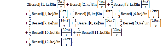
etc., etc. So the solution becomes a tedious accounting of the sum of all the sums. To make the calculation easier we should find a mathematics program, Mathematica for instance, which will call up Bessel’s functions as subroutines. For that particular program, here is the code: |
|
where Psi[t_] is the function to be calculated, namely, ψ(t); BesselJ[k,kε]is the Bessel function subroutine for Jk(kε); this is multiplied by the sine function, Sin[k2πt/τ]; and the bracket {k,1,12} sets the limits of index for the sum from k = 1 to k = 12.
In Mathematica, if we input this code: |
|
this output will be returned: |
|
Specifying the value for ε will cause the program to calculate and return a result which, if then added to 2πt/τ, will give the function ψ(t). |
|
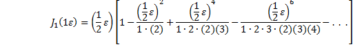
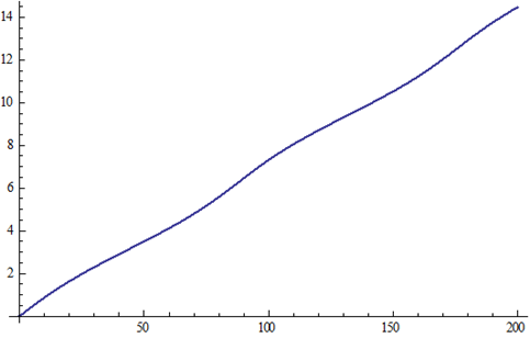
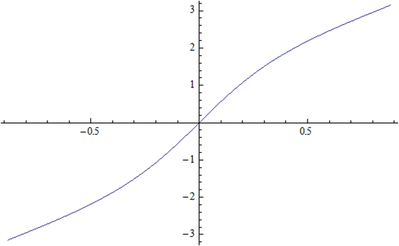
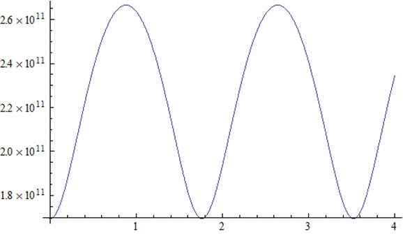
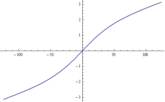
Mercury This Mathematica code produces graphs for ψ(t), θ(t) and r(t):
"Mercury" ε = .2056 m = (2 * 3.1415926 t)/87.969 a = 57871000000
psi[t_] = m + Sum[(2/k)*BesselJ[k,k*ε ]Sin[k*m],{k,1,12}] Plot[psi[t],{t,0,200}]
theta[t_] = 2*ArcTan[Sqrt[(1+ε)/(1-ε)]*Tan[psi[t]/2]] Plot[theta[t],{t,-87.969/2,87.969/2}]
r[t_] = a*(1-ε*ε)/(1+ε*Cos[theta[t]]) Plot[r[t],{t,0,200}] |
|
Notes on Mathematica code:
a) In using the notation psi[t_], the blank space underline is required when defining the function on the left-hand-side of the equal sign. Drop the blank space underline when using the function in calculations. b) All subroutines and embedded functions in Mathematica must have upper case first letter, for example, Sin, Tan, ArcTan, Sqrt, etc., and their arguments must be placed in square brackets. c) The bracket {t,0,200} in the Plot command places the variable, t, on the x-axis, and sets the minimum (0) and maximum (200) limits of the x-axis. The y-axis is auto-scaled with this command. d) A right-arrow is generated by a minus sign followed by a greater-than sign: -> e) There are many ways to go wrong in Mathematica. If for some (unknown) reason these short programs do not work as exactly written here, you’ll just have to figure out Mathematica for yourself — as you should anyway, of course.
Those commands produce these results for: |
|
Mercury |
|
\\\\\\\\\\\\\\\\\\\\\\\\\\\\\\\\\\\\\\\\\\\\\\\\\\\\\\\\\\\\\\\\\///////////////////////////////////////////////////////////////// |
|
ψ(t) versus t |
|
θ(t) versus t |
|
r(t) versus t |
|
Mars |
|
Mathematica code for Mars:
"Mars" ε = .0934 m = 2 * 3.1415926 t /1.8809 "years" a = 1.5237*149500000000 "AU * meter/AU"
psi[ε_,m_] = m + Sum[(2/n)*BesselJ[n,nε]Sin[n*m],{n,1,12}] Plot[psi[ε,t],{t,0,2}]
theta[t_] = 2*ArcTan[Sqrt[(1+ε)/(1-ε)]*Tan[psi[ε,m]/2]] Plot[theta[t],{t,-1.88/2,1.88/2}]
r[t_] = a*(1-ε*Cos[psi[ε,m]]) Plot[r[t],{t,0,4}] |
|
ψ(t) versus t |
|
θ(t) versus t |
|
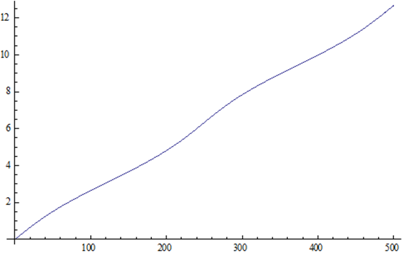
Halley’s Comet Fact Sheet
Aphelion 35.1 AU * 1.495x1011m/AU = 5.247x10¹² m Perihelion .586 AU* 1.495x1011m/AU = 8.761x10¹⁰ m eccentricity ε = .967 Period τ = 75.3 year Mass = 2.2x10¹⁴ kg For a smooth curve this orbit requires many terms in the sum of Bessel’s functions n = number of terms
Note that the eccentricity is quite high. |
|
r(t) versus t |
|
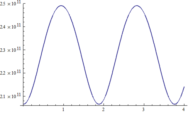
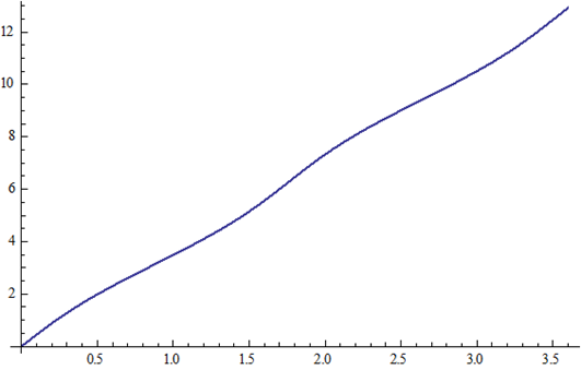
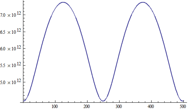
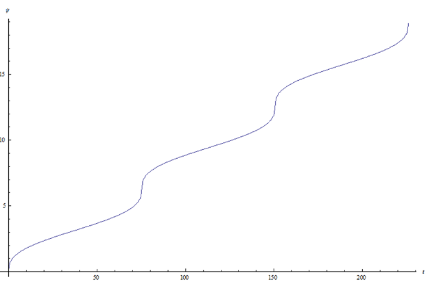
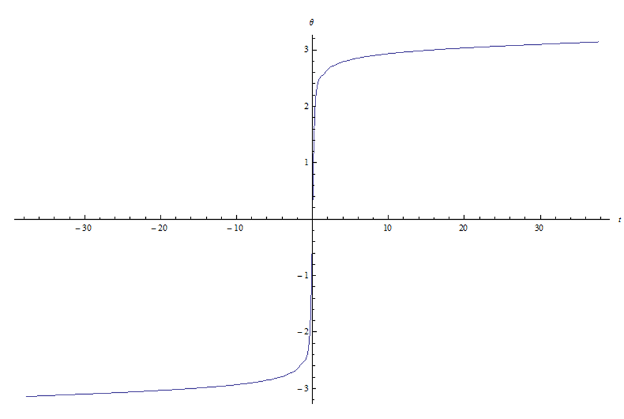
Eros the asteroid |
|
Mathematica code for Eros:
"Eros" ε = .2230 m = 2*3.1415926 t / 1.761 "years" a = 1.4583*149500000000 "AU * meter/AU"
psi[ε_,m_] = m + Sum[(2/n)*BesselJ[n,n*ε]Sin[n*m],{n,1,12}] Plot[psi[ε,t],{t,0,3.6}]
theta[t_] = 2*ArcTan[Sqrt[(1+ε)/(1-ε)]*Tan[psi[ε,m]/2]] Plot[theta[t],{t,-1.761/2,1.761/2}]
r[t_] = a*(1-ε*ε)/(1+ε*Cos[theta[t]]) Plot[r[t],{t,0,4}] |
|
ψ(t) versus t |
|
θ(t) versus t |
|
r(t) versus t |
|
Pluto |
|
ψ(t) versus t |
|
θ(t) versus t |
|
r(t) versus t |
|
Halley’s Comet |
|
Mathematica code for Halley’s Comet:
"Halley's Comet" "ε eccentricity" ε = .967 "tau Period" tau = 75.3 m = 2*π*t /tau "a semi-major axis" a = 17.8*149500000000 "requires many terms for smooth curve" "n = number of terms in Bessel's Function" n = 48
"Sum[2/kBesselJ[k,k ε]Sin[k m],{k,1,n}]" psi[t_] = m+Sum[2/k BesselJ[k,k ε]Sin[k m],{k,1,n}] Plot[psi[t],{t,0,3*tau},AxesLabel->{t,ψ}]
theta[t_] = 2*ArcTan[Sqrt[(1+ε)/(1-ε)]*Tan[psi[t]/2]] Plot[theta[t],{t,-tau/2,tau/2},AxesLabel->{t,θ}]
r[t_] = a*( 1-ε*ε)/(1+εCos[theta[t]]) Plot[r[t],{t,0,3*tau},AxesLabel->{t,r}] |
|
ψ(t) versus t |
|
θ(t) versus t |
|
r(t) versus t |
|
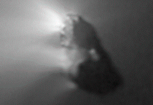
Halley’s Comet, the nucleus |
|
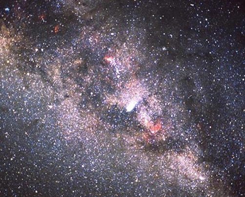
Haley’s Comet, with Milky Way background |

|
C) Trial and error
Consider a hypothetical planet with period τ = 100 days and eccentricity ε = .25, with our clock set such that t = 0 occurs when the planet is at perihelion. Let the semi-major axis be a = 5x10⁹ m. Use Kepler’s equation in this form: |
|
1) How far along in its orbit is the planet after a time of t = 50 days? |
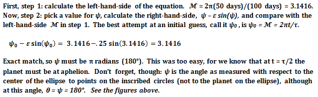
|
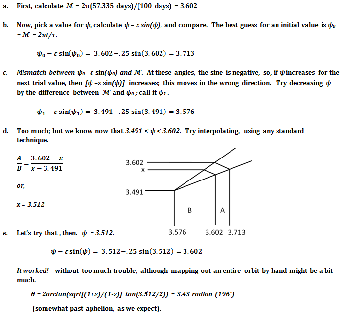
2) How far along is this same planet after a time of t = 57.335 days? |
|
3) How far along is the planet at i) t = 17.126 days, and at ii) t = 25 days? We leave this as an exercise, for the reader will be greatly edified by calculating ψ, θ, and r for each of the specified times. |
|
Kepler’s Equation, Part 2 |
|
webpages and Eos image copyright 2015 M Nealon |
|
Top Kepler’s Equation |
|
Page 1 Elliptical Orbits |
|
Page 2 Time in Orbit |
|
Kepler’s Equation, Part 2 |