
|
EOS |


|
Various Topics |
|
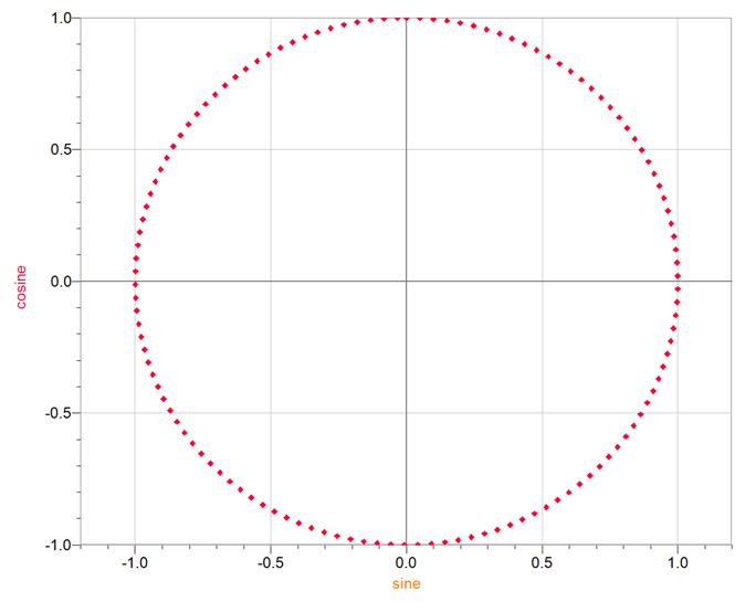
A parametric representation of a relationship between n variables uses an extra variable— called a parameter—to couple the variables in n equations. The set of numbers over which the parameter varies is its domain. Of course parametric representations are not unique; any number of parametric forms might be found for a given curve. Parametric equations are not limited to two variables, but perhaps it might be easier to see in a plane curve. In two dimensions write x and y as functions of the parameter t. Let x = x(t) and y =y(t). Consider this example: x = sin(t) y = cos(t) This is the parametric representation of a unit circle. In this case, that the equation describes a circle can be seen easily if you square both equations, then add them together. Use the trigonometric identity sine squared plus cosine squared equals one, to obtain x^2 + y^2 = 1. This is the equation for a circle. The question is: How does one graph the parametric form of a circle in in Cartesian coordinates? |
How to Graph a Parametric Representation of a Curve |
|
For a circle of radius r, x = r sin(t) y = r cos(t) |
|
To graph by hand you would begin by getting a piece of graph paper and making a table of x- and y-values: select an arbitrary value for t, calculate both x and y and enter them in the table. Continue across the domain of t. As you plot the (x,y) points, the curve begins to take shape. Make a graph on the computer in the same manner. Solve both equations in the parameter t, plot one of the equations along the y-axis and the other equation along the x-axis. In the case of the circle of unit radius above it does not matter along which axis the sine or cosine is placed.
|
|
In Logger-Pro
In order to generate the parameter values, first click on “Data” at the top bar and then click on “New Manual Column”. Under “Name” enter the parameter name: t. Click “Generate Values” under the “Column Definition” tab. Since the parameter t will range from 0 to 2π for a circle, set the “Start:” value at 0 and the “End:” value at 6.28. Select a small number for the “Increment:”. Then click “Done”. Click on “Data” at the top bar and then click on “New Calculated Column”. Under “Name” enter “cosine”. Put the cursor in the “Equation” box and click once. Now click on the “Functions” box and roll down to “trigonometric” and click on “cos”. The cosine function will appear in the “Equation” box. The cursor should be inside the parentheses; then click “Variables (Columns)”. Select “t” and it will appear inside the parentheses. Click “Done” and the values of cos(t) will appear in a new column of data called “cosine”. Click on “Data” at the top bar and repeat this using the name “sine” and place in the “Equation” box the function sin(“t”). The thing about the “Equation” box is that it won’t recognize t as a variable if you just type it into the equation. The program recognizes variables in columns only. To place the data points on the graph, first put the cursor on the graph itself and double click. The ”Graph Options” box will appear on the graph. The same box can be accessed by clicking on “Options” at the top bar and selecting “Graph Options”. In this box, find “Y-axis Options”, place the cursor in the little box next to “cosine” and click once. This tells the program what to place on the y-axis. Find the area labeled “X-axis” and the drop-down box “Column”. Click on “sine” to place this column on the x-axis. Click “Done”. The data will not look like a circle because the x-axis, now sine-axis and the y-axis, now cosine-axis are on the same scale but the graph is not square. Place the cursor on the graph itself, and double click to open the “Graph Options” box. Find the “Scaling” drop down boxes for both the x and y axes. In both, click on “Manual”. Leave “1.0” at the top and “–1.0” at the bottom along the y-axis; set the x-axis to “-1.2” in the “Left:” box and 1.2” in the “Right:” box. This will make the circle approximately round. The data points will have the same color as whatever is placed on the y-axis. To change the size or shape of the data points, double click on the word “cosine” under the “Data Set” box. This will open he “Calculated Column Options” box. Now click on the “Options” tab. Select whichever “Point Protector” “Style” is appropriate, select the size and color. To increase or decrease the number of data points double click on the t at the top of the column of data under “Data Set”. The “Manual Column Options” box will open; click on “Generate Values” again. The increment value now can be changed. |
|
An ellipse is given by x = a sin(t) y = b cos(t) for a ≠ b |
|
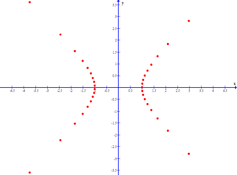
The parametric representation of both branches of a hyperbola is x(t) = a sec(t) y(t) = b tan(t) Where a and b are constants which determine the shape of the hyperbola. Sec(t) is the secant function and tan(t) is the tangent function. |
|
In Graph Graph is easier to use than Logger Pro in a lot of respects. Find the “Insert a new function” icon at the top bar. It looks like a set of blue, crossed axes with a red curve. Click once on this icon to open the “Insert function” box. At the top of the box, click the “Function type” down-arrow and select “Parametric function x(t), y(t)”. Under “Function equation”, enter sec(t) in the “x(t)” box and tan(t) in the “y(t)” box. In the “Argument range” box, set the domain of the parameter from –6.28 to 6.28 and the number of steps to, say, 42. Under the “Graph properties” box at the bottom, change “Automatic” to “Dots” and give the dots a width of 8. Click “OK” to place the points on the graph. The x– and y–axes are not on the same scale. Click on the word “Zoom” at the top bar, then click on “Square”. The axes will now appear symmetric. |
|
Hyperbola in Cartesian form x^2 y^2 = 1 a^2 b^2 |
|
For a single branch hyperbola x = a cosh(t) y = b sinh(t) |
|
To place the hyperbolas open-up and open-down, make the switch: x(t) = a tan(t) y(t) = b sec(t) |
|
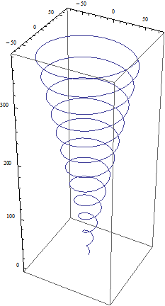
For a circular helix, set a= b |
|
A linear coiled spring generally has the shape of a right-circular helix. Imagine that each loop of the spring is approximately in a plane, then the helix is said to be “right circular” if all of the planes are parallel, all loops have the same radius and the centers of all loops fall on a straight line which is perpendicular to the planes of the loops. A right-elliptical helix in three dimensional parametric form can be written as x(t) = a cos(t) y(t) = b sin(t) z(t) = t where a and b are the semi-major and semi-minor axes. For a, b both positive the helix is said to be “right-handed”. For a left-handed coil, either a or b but not both, should be negative. A linearly tapering, or conical, helix is given by x(t) = t cos(t) y(t) = t sin(t) z(t) = t The t which multiplies the trig functions causes the linear taper. An elliptical conical helix may be obtained if x(t) and y(t) are multiplied by non-equal constants. |
|
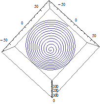
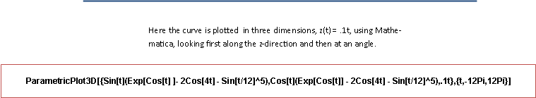
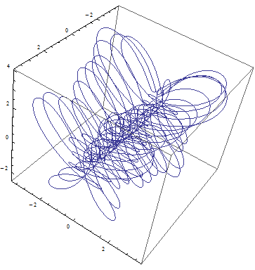
In Mathematica Mathematica has an enormous number of rules, any one of which, if violated, will prevent the successful execution of a plot. A three dimensional parametric plot can be generated by the Mathematica function “ParametricPlot3D[ { x(t) , y(t) , z(t) }, { t, tmin, tmax } ]”. The outside brackets, which must be square, enclose all details of the required plot: the function to be graphed, the scale, colors, etc.; each detail must be inside a set of curly brackets and each set of brackets must be separated by a comma. The manner of entering the parametric function is shown, but none of the other details are given here. Without these other details being specified, the program uses default values. The three dimensional parametric function to be graphed, placed within curly brackets (shown here in bold only for the purpose of illustration) must be entered in the order x(t) , y(t) , z(t) , and be separated by commas. The name of the parameter and the limits of its domain must be placed within their own set of curly brackets. Here is an example of a conical helix: ParametricPlot3D[ { t Cos[t] , t Sin[t] , 5t} , {t,0,24Pi} ] The trig functions must be capitalized and their arguments must be in square brackets. The “5t” produces a strong taper. The domain ranges from 0 to 24π, giving 12 loops. |
|
Looking in the direction of positive z. Notice the “right-handedness” of the helix. If the thumb of the right hand points in the direction of +z, then the fingers point along the curve and curl in the direction of increasing t. |
|
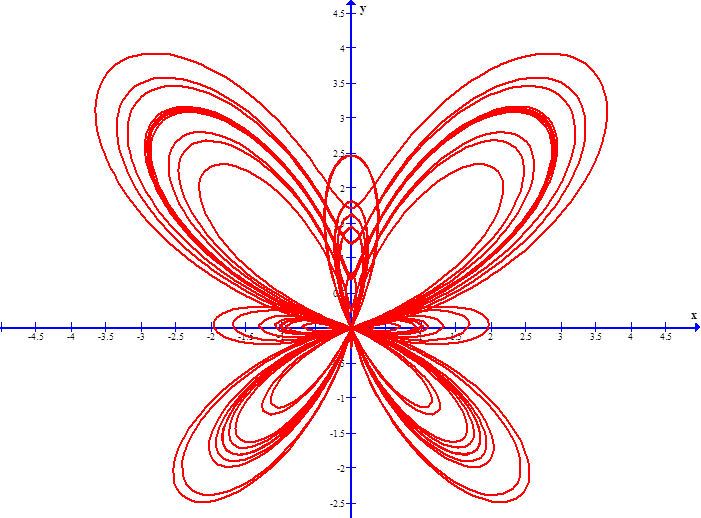
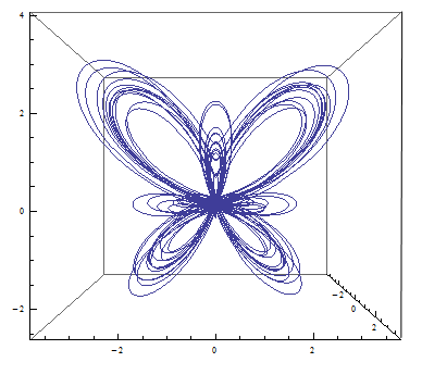
This is the so-called “Butterfly” curve: x(t) = sin(t) {exp[ cos(t) ] - 2cos(4t) - sin(t/12)^5 }
y(t) = cos(t) {exp[ cos(t) ] - 2cos(4t) - sin(t/12) ^5 }
The notation sin(t/12)^5 means ”raise the sine of t /12 to the fifth power”.
Shown here in Graph, the domain of t is from –12π to +12π, and the line width is 2. |
|
webpages and Eos image copyright 2010 M Nealon |